To examine the performance of the M66's DAC, I used the coaxial and optical S/PDIF inputs, both of which accepted data sampled at rates up to 192kHz, and network data sourced from Roon.
The NAD's digital inputs preserved absolute polarity at the balanced and unbalanced outputs but inverted polarity at the headphone output. With the volume control set to its maximum, the M66's output level with a full-scale 1kHz tone was 5.28V balanced, 2.64V unbalanced, and 7.93V headphone. The M66's DAC offers a well-managed gain architecture.
The appropriate word to describe the measured performance of the NAD M66's line, phono, and digital inputs is "superb." The company has some serious audio engineering talent in-house.—John Atkinson
Footnote 1: I have been asked why I use this particular undithered signal. In the twos-complement encoding used by 16-bit digital audio, –1 least significant bit (LSB) is represented by 1111 1111 1111 1111, digital zero by 0000 0000 0000 0000, and +1 LSB by 0000 0000 0000 0001. If the waveform is symmetrical, this indicates that changing all 16 bits in the digital word gives exactly the same change in the analog output level as changing just the LSB.
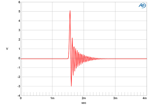
Fig.12 NAD M66, network input, impulse response (one sample at 0dBFS, 44.1kHz sampling, 4ms time window).
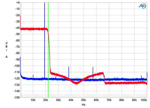
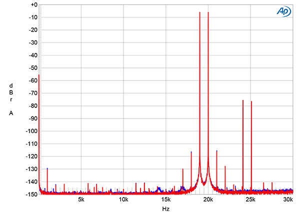
Fig.13 NAD M66, network input, wideband spectrum of white noise at –4dBFS (left channel red, right magenta) and 19.1kHz tone at 0dBFS (left blue, right cyan) into 100k ohms with data sampled at 44.1kHz (20dB/vertical div.).
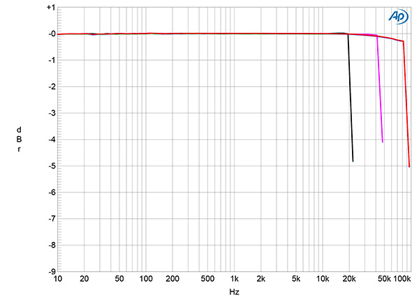
Fig.14 NAD M66, digital inputs, frequency response at –12dBFS into 100k ohms with data sampled at: 44.1kHz (left channel green, right gray), 96kHz (left cyan, right magenta), and 192kHz (left blue, right red) (1dB/vertical div.).
Fig.12 shows the M66's impulse response with network data sampled at 44.1kHz. The filter is a minimum-phase type with all the ringing following the single sample at 0dBFS. The magenta and red traces in fig.13 show the filter's ultrasonic rolloff with 44.1kHz white noise data at –4dBFS. They reach full stop-band attenuation just above half the sample rate (this indicated by the vertical green line), with the aliased image at 25kHz of a full-scale tone at 19.1kHz (cyan, blue) completely suppressed. (Peculiarly, when I repeated this test with TosLink data, the aliased image at 25kHz was suppressed by 70dB rather than completely—see fig.18—even though with optical data the white noise spectrum and impulse response were identical.) The frequency response with 44.1kHz, 96kHz, and 192kHz data is flat in the audioband, with a sharp rolloff just below half of each sample rate (fig.14).
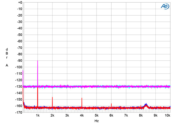
Fig.15 NAD M66, digital inputs, spectrum with noise and spuriae of dithered 1kHz tone at –90dBFS with: 16-bit data (left channel cyan, right magenta), 24-bit data (left blue, right red) (20dB/vertical div.).
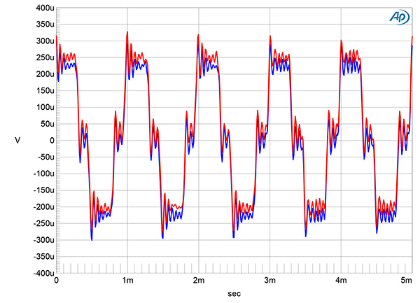
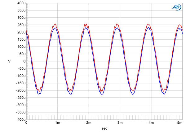
Fig.16 NAD M66, digital inputs, waveform of undithered 1kHz sinewave at –90.31dBFS, 16-bit data (left channel blue, right red).
Fig.17 NAD M66, digital inputs, waveform of undithered 1kHz sinewave at –90.31dBFS, 24-bit data (left channel blue, right red).
An increase in bit depth from 16 to 24, with dithered data representing a 1kHz tone at –90dBFS, dropped the M66's noisefloor by 33dB (fig.15). This implies a measured resolution of 22 bits, one of the highest I have found. When I played undithered data representing a tone at exactly –90.31dBFS (footnote 1), the waveform was symmetrical, with negligible DC offset. The three DC voltage levels described by the data were clearly defined (fig.16). With undithered 24-bit data (fig.17), the M66 output a superbly clean sinewave.
Fig.18 NAD M66, 24-bit TosLink data, HF intermodulation spectrum, DC–30kHz, 19+20kHz at 0dBFS into 100k ohms, 44.1kHz data (left channel blue, right red; linear frequency scale).
As it had with the analog inputs, the NAD's digital inputs produced very low levels of distortion. Fig.13 showed that the harmonics associated with the 19.1kHz tone all lay below –100dB. Intermodulation distortion with optical data representing an equal mix of 19 and 20kHz tones, each at –6dBFS, was also very low (fig.18).
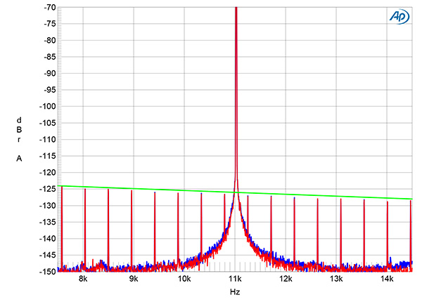
Fig.19 NAD M66, 16-bit network data, high-resolution jitter spectrum of analog output signal, 11.025kHz at –6dBFS, sampled at 44.1kHz with LSB toggled at 229Hz (left channel blue, right red). Center frequency of trace, 11.025kHz; frequency range, ±3.5kHz.
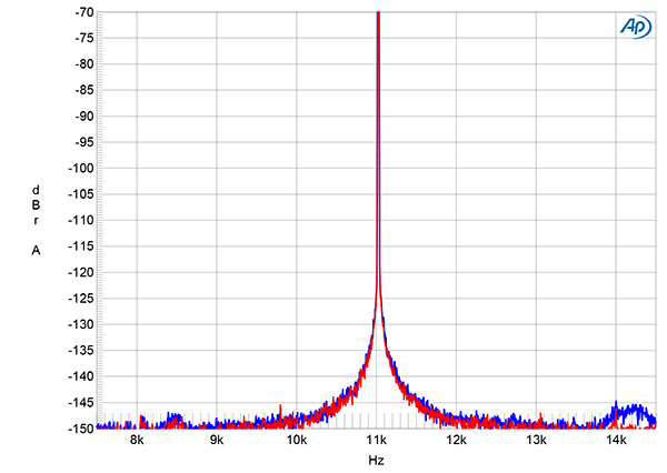
Fig.20 NAD M66, 24-bit network data, high-resolution jitter spectrum of analog output signal, 11.025kHz at –6dBFS, sampled at 44.1kHz with LSB toggled at 229Hz (left channel blue, right red). Center frequency of trace, 11.025kHz; frequency range, ±3.5kHz.
Fig.19 shows the spectrum of the M66's output when it was fed 16-bit J-Test data via Roon. All the odd-order harmonics of the undithered low-frequency, LSB-level squarewave lie at the correct levels, though the central spike that represents the high-level tone at one-quarter the sample rate (Fs/4) is broadened at its base. This implies the presence of low-frequency random jitter, though at a low level. Repeating this analysis with 24-bit J-Test data via my network and with 16- and 24-bit S/PDIF J-Test data gave identical results (fig.20).
Footnote 1: I have been asked why I use this particular undithered signal. In the twos-complement encoding used by 16-bit digital audio, –1 least significant bit (LSB) is represented by 1111 1111 1111 1111, digital zero by 0000 0000 0000 0000, and +1 LSB by 0000 0000 0000 0001. If the waveform is symmetrical, this indicates that changing all 16 bits in the digital word gives exactly the same change in the analog output level as changing just the LSB.