Sidebar 3: Measurements
I used DRA Labs' MLSSA system and a calibrated DPA 4006 microphone to measure the KEF Blade Two's frequency response in the farfield, and an Earthworks QTC-40 for the nearfield and spatially averaged room responses. The Blade Two's voltage sensitivity is specified as 90dB/2.83V/m; my estimate was somewhat lower than this, at 87.1dB(B)/2.83V/m. The Blade Two's nominal impedance is 4 ohms, with a minimum value of 3.2 ohms. My measurement (fig.1) revealed a minimum magnitude (including cable) of 3.4 ohms at 177Hz (solid trace). Though the impedance remained below 6 ohms in the midrange, the electrical phase angle (dashed trace) was low in the same region. The phase angle was greater in the treble region but the impedance was also higher, ameliorating any drive difficulty.
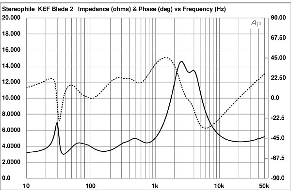
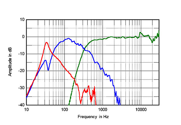
 The saddle centered just below 40Hz in the impedance-magnitude trace in fig.1 suggests that the two ports on the rear panel are tuned in this region. The minimum-motion notch at 37Hz in the sum of the woofers' nearfield outputs (fig.3, blue trace; all four woofers behave identically) confirms that this is the port tuning frequency. Both ports appear to behave identically, and the sum of their nearfield responses (fig.3, red trace) peaks sharply between 30 and 40Hz, with a smooth rollout above that region broken only by some very low-level peaks in the midrange. Unusually, the woofers and ports appear to roll off below the port resonance with closer to 18dB/octave slopes rather than the 12dB/octave slope typical of a ported design. This is because the ports are tuned lower than with a textbook B4 alignment, which gives an initial third-order rolloff that shallows off to 12dB/octave at very low frequencies.
 While capturing these in-room responses, I was impressed by how closely the two review samples matched. Other than the left speaker having slightly more output in a narrow band in the presence region, the two channels matched to within 0.5dB from 600Hz to 30kHz (fig.8).
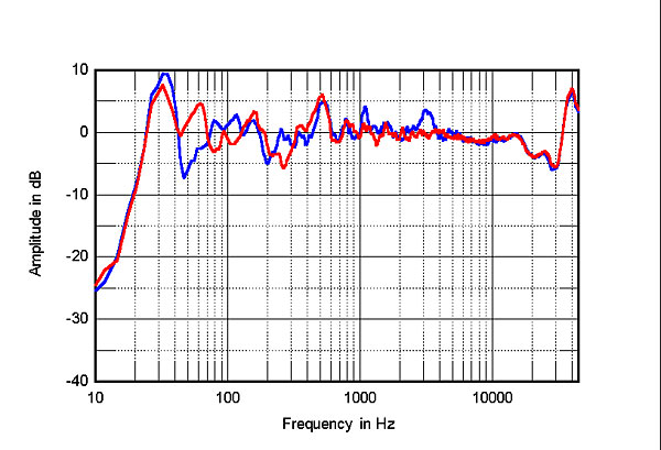
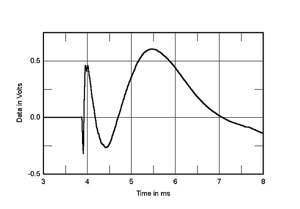
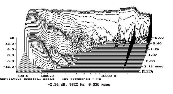
Fig.1 KEF Blade Two, electrical impedance (solid) and phase (dashed) (2 ohms/vertical div.).
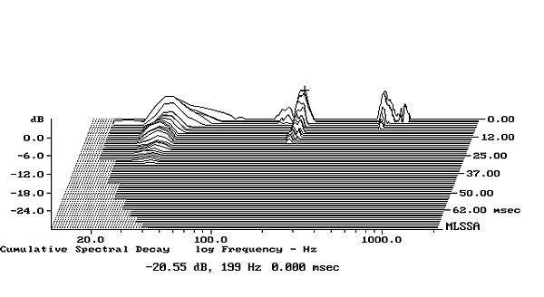
Other than one at 30kHz, presumably due to the tweeter's fundamental dome resonance, the traces in fig.1 are free from the small discontinuities that would indicate the presence of enclosure panel resonances. When I investigated the behavior of the cabinet with a simple plastic-tape accelerometer (similar to a piezoelectric acoustic-guitar pickup), I found very little untoward. The only resonant mode I could find was at 200Hz (fig.2), and although it was present on the curved baffle and sidewalls, it was very low in level. The Blade Two's enclosure is extremely inert, and the force-canceling woofer arrangement seems to work as advertised.
Fig.2 KEF Blade Two, cumulative spectral-decay plot calculated from output of accelerometer fastened to center of front baffle below bottom woofer (MLS driving voltage to speaker, 7.55V; measurement bandwidth, 2kHz).
Fig.3 KEF Blade Two, acoustic crossover on tweeter axis at 50", with nearfield responses of midrange unit (green), woofers (blue) and ports (red).
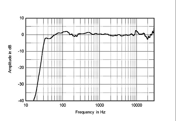
Higher in frequency in fig.3, the woofers roll off smoothly, crossing over to the midrange section of the Uni-Q driver (green trace) between 300 and 400Hz. The midrange unit also rolls off below the crossover to the woofers with an 18dB/octave slope, and its crossover to the coaxial tweeter is seamless. While there is a small peak at 10kHz, note how smooth, even, and extended the Blade Two's upper-frequency response otherwise is in this graph. Fig.4 shows the KEF's farfield response on the tweeter axis, averaged across a 30° horizontal window and spliced at 300Hz to the complex sum of the nearfield responses of the midrange unit, woofers, and ports (taking into account acoustic phase and the different distance of each radiator from a nominal farfield microphone position). The Blade Two offers a superbly flat, even response on the tweeter axis. Wow!
Fig.4 KEF Blade Two, anechoic response on tweeter axis at 50", averaged across 30° horizontal window and corrected for microphone response, with complex sum of nearfield responses plotted below 300Hz.
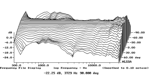
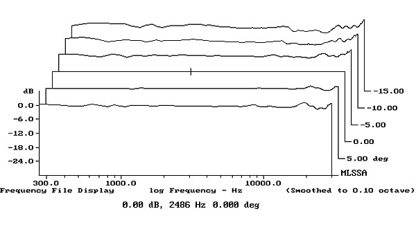
That doesn't in itself mean that the speaker will sound neutral, as the perceived quality will also depend on the radiation pattern. The KEF's horizontal pattern is shown in fig.5, normalized to the response on the tweeter axis, which is therefore presented as a straight line (which is not too different from the actual response). Other than the cancellation notch between 300 and 400Hz and the boost centered on 1kHz at extreme off-axis angles, due to destructive interference between the woofers on opposed sides of the enclosure, the contour lines in this graph are superbly smooth and even. The horizontal dispersion is narrower in the midrange and lower treble than with a conventional dynamic loudspeaker, but wider in the top octave. In the vertical plane (fig.6), the Blade Two's response hardly varies at all over a wide (±10°) window centered on the tweeter axis, which itself is 39" from the floor.
Fig.5 KEF Blade Two, lateral response family at 50", normalized to response on tweeter axis, from back to front: differences in response 90–5° off axis, reference response, differences in response 5–90° off axis.
Fig.6 KEF Blade Two, vertical response family at 50", normalized to response on tweeter axis, from back to front: differences in response 15–5° above axis, reference response, differences in response 5–10° below axis.
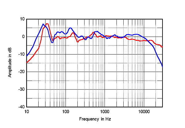
The red trace in fig.7 is the Blade Two's spatially averaged, 1/6-octave response at the listening position in my room. (Using an Earthworks QTC-40 microphone, I average 20 1/6-octave–smoothed spectra, individually taken for the left and right speakers using SMUGSoftware's FuzzMeasure 3.0 program and a 96kHz sample rate, in a rectangular grid 36" wide by 18" high and centered on the positions of my ears.) Other than the large peak between 30 and 40Hz, due to the coincidence of the port tuning frequency and the lowest mode in my room, and which I couldn't eliminate by experimenting with the speaker positions, the KEFs' in-room response is impressively smooth and even from the midbass through the high treble. The blue trace in this graph is a similar spatially averaged response for the DALI Rubicon 8 speakers, which I reviewed in the March issue. That Danish speaker produced more upper-bass energy in-room, which balanced its higher level of mid-treble energy, and extended slightly lower in frequency.
Fig.7 KEF Blade Two, spatially averaged, 1/6-octave response in JA's listening room (red); and of DALI Rubicon 8 (blue).
Fig.8 KEF Blade Two, 1/6-octave response in JA's room at listening position (left speaker blue, right red).
In the time domain, the Blade Two's step response on its tweeter axis (fig.9) indicates that the tweeter is connected in inverted acoustic polarity, the midrange and woofers in positive acoustic polarity. More important, the decay of the tweeter's step smoothly blends with the rise of the midrange unit's step, and the decay of that unit's step smoothly blends with the rise of the woofers' step. This suggests optimal crossover design. Finally, the KEF's cumulative spectral-decay plot on the tweeter axis (fig.10) demonstrates superbly clean decay from the midrange upward.
Fig.9 KEF Blade Two, step response on tweeter axis at 50" (5ms time window, 30kHz bandwidth).
Fig.10 KEF Blade Two, cumulative spectral-decay plot on tweeter axis at 50" (0.15ms risetime).
KEF's Blade Two offers superb measured performance that is close to the state of the art.—John Atkinson