Sidebar 3: Measurements
I used DRA Labs' MLSSA system, a calibrated DPA 4006 microphone, and an Earthworks microphone preamplifier to measure the Q Acoustics 5040's quasi-anechoic behavior in the farfield. (The 5040's manual doesn't mention an optimal listening axis, so I examined the farfield frequency- and time-domain responses on the tweeter axis.) I used an Earthworks QTC-40 mike for the nearfield and in-room responses and Dayton Audio's DATS V2 system to measure the impedance magnitude and electrical phase angle.
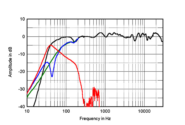
With the port open, their response, measured in the nearfield (fig.3, blue trace), has the expected minimum-motion notch at 43Hz. The red trace in fig.3 shows the nearfield output of the port; it peaks slightly below the tuning frequency and its upper-frequency rollout is clean, with an increase in the low-pass rate above 170Hz. With the port sealed, the response of the woofers (fig.3, green trace) gently rolls off below 100Hz. Both the woofers' response and the complex sum of the woofer and port responses (fig.3, black trace below 300Hz) have a small suckout centered at 173Hz. This coincides with the frequency at which the port's rolloff increases, suggesting that some sort of internal anti-resonance is present. As with the Concept 50, there is little sign of the usual peak in the midbass region due to the nearfield measurement technique, which assumes that the drive units are mounted in a true infinite baffle. The speaker's reflex alignment is therefore overdamped, which implies that the speaker will give the highest low-frequency output when it is placed relatively close to the wall behind it.
The Q Acoustics 5040 offers generally excellent measured performance. However, that demanding impedance might make amplifier choice problematic, and the extended high frequencies will mean experimentation with toe-in might be necessary to optimize the speakers' treble balance.—John Atkinson
Footnote 1: Every time I measure a loudspeaker, I also measure one my 1970s-vintage LS3/5a's to make sure that a systematic error hasn't occurred. Footnote 2: EPDR is the resistive load that gives rise to the same peak dissipation in an amplifier's output devices as the loudspeaker. See "Audio Power Amplifiers for Loudspeaker Loads," JAES, Vol.42 No.9, September 1994, and stereophile.com/reference/707heavy/index.html.
Footnote 3: Using the FuzzMeasure 3.0 program, a Metric Halo MIO2882 FireWire-connected audio interface, and a 96kHz sample rate, I average 20 1/6-octave–smoothed spectra, individually taken for the left and right speakers, in a rectangular grid 36" wide by 18" high and centered on the positions of my ears.
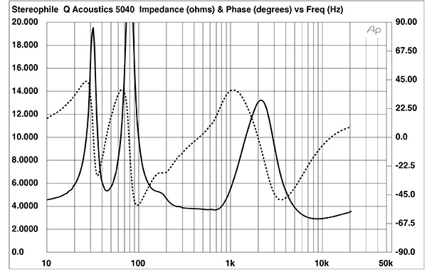
Fig.1 Q Acoustics 5040, electrical impedance (solid) and phase (dashed) with port open (2 ohms/vertical div.).
Q Acoustics specifies the 5040's voltage sensitivity as a high 91.5dB/2.83V/m. My estimate, calculated by comparing the SPL at 50" of the 5040 with that produced by a Rogers LS3/5a (footnote 1), was within experimental error of the specified figure, at 91.7dB(B)/2.83V/m. The 5040's impedance is specified as 6 ohms, with a minimum value of 3 ohms. With the port on the rear panel sealed with the supplied foam plug, the impedance was typical of a sealed enclosure, with a relatively high tuning frequency of 69Hz. With the port open, the impedance magnitude (fig.1, solid trace) varied between 4 ohms and 13 ohms over most of the audioband, with minimum values of 3.7 ohms at 560Hz and 2.91 ohms at 8.7kHz. The electrical phase angle (dotted trace) is often high, reaching –53° at 96Hz and +37° at 1084Hz. As a result, the effective resistance, or EPDR (footnote 2), lies below 3 ohms over much of the audioband, with minimum values of 2 ohms between 131Hz and 210Hz, 1.79 ohms at 836Hz, and 1.35 ohms at 5.8kHz. This loudspeaker is a difficult load.
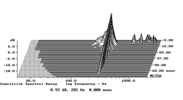
Fig.2 Q Acoustics 5040, cumulative spectral-decay plot calculated from output of accelerometer fastened to center of back panel (MLS driving voltage to speaker, 7.55V; measurement bandwidth, 2kHz).
When I investigated the enclosure's vibrational behavior with a plastic-tape accelerometer, I found a resonant mode at 285Hz that was present on all the panels. Its amplitude was lowest on the front baffle below the drive units and strongest on the rear panel (fig.2). This mode has a relatively high Q (quality factor) and its frequency lies between the notes C# and D in the equal-tempered scale. Both these factors will reduce the possibility of this resonance having audible consequences. (A resonance needs to be stimulated at its exact frequency by the same number of cycles as its Q to be fully excited.) The two woofers behaved identically.
Fig.3 Q Acoustics 5040, anechoic response on tweeter axis at 50", averaged across 30° horizontal window and corrected for microphone response, with the nearfield responses of the woofers (blue), port (red), their complex sum (black), and the nearfield sealed-box woofer response (green), respectively plotted below 300Hz, 700Hz, 300Hz, and 300Hz.
The black trace above 300Hz in fig.3 shows the 5040's quasi-anechoic farfield response, averaged across a 30° horizontal window centered on the tweeter axis and taken without the grille. The response is relatively even overall, though there is a slight shelf in the upper midrange and low treble. The pair matching between the two samples was excellent, the difference in the farfield response falling within ±0.25dB limits from 1kHz to 15kHz. The response with the grille (not shown) was very similar in the audioband, other than introducing some small, narrow suckouts between 5kHz and 10kHz. The grille also reduced the level of the slight peak at 20kHz by 2dB.
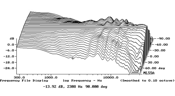
Fig.4 Q Acoustics 5040, lateral response family at 50", normalized to response on tweeter axis, from back to front: differences in response 90–5° off axis, reference response, differences in response 5–90° off axis.
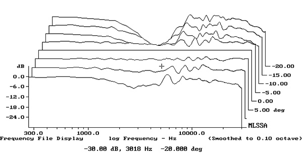
Fig.5 Q Acoustics 5040, vertical response family at 50", normalized to response on tweeter axis, from back to front: differences in response 20–5° above axis, reference response, differences in response 5–15° below axis.
Fig.4 shows the 5040's horizontal dispersion, normalized to the response on the tweeter axis, which thus appears as a straight line. The contour lines in this graph are even, though the radiation pattern narrows slightly at the top of the woofers' passband. The dispersion is wider in the region covered by the tweeter. Fig.5 shows the speaker's dispersion in the vertical plane, again normalized to the response on the tweeter axis. The response is maintained 5° above the tweeter axis, which is useful considering that the tweeter is 30" from the floor. A suckout starts to develop in the crossover region 10° above the reference axis.
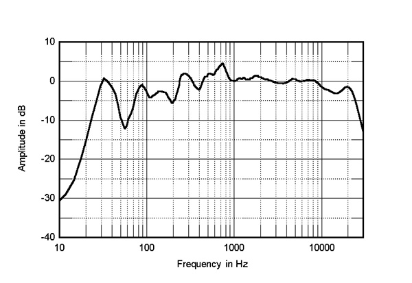
Fig.6 Q Acoustics 5040, spatially averaged, 1/6-octave response in JA's listening room.
Fig.6 shows the Q Acoustics 5040s' spatially averaged response (footnote 3) in my room with their ports open and without the grilles. The response is reasonably even above 230Hz, though with a slight excess of energy in the upper midrange. There is insufficient upper- and midbass energy due, presumably, to the fact that I wasn't able to move the speakers as close to the wall behind them as necessary. Instead of the in-room response gently sloping down above 3kHz, which will be due to the increased absorption of the room's furnishings as the frequency increases, the 5040s' response remains at full level up to 9kHz.
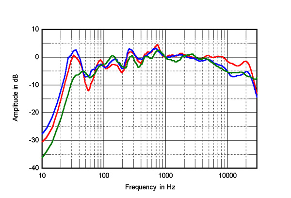
Fig.7 Q Acoustics 5040, spatially averaged, 1/6-octave response in JA's listening room (red), of the Q Acoustics Concept 50 (blue), and of the KEF LS50 (green).
For reference, the red trace in fig.7 repeats the spatially averaged response of the 5040s and adds that of the Q Acoustics Concept 50s (blue trace) and that of my long-term reference KEF LS50s (green trace). The two Q Acoustics speakers have a very similar in-room response in the bass, where the two models excite the lowest-frequency mode in my room to the same extent, and the midrange. However, the 5040s' spatially averaged response has more energy above 5kHz, while the Concept 50s' response was almost identical to that of the KEFs in this region.
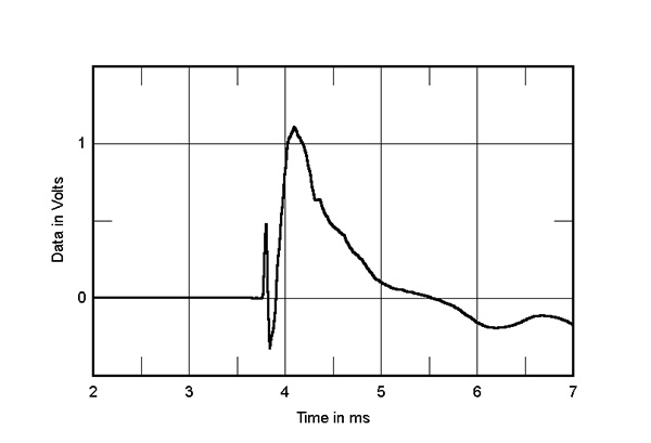
Fig.8 Q Acoustics 5040, step response on tweeter axis at 50" (5ms time window, 30kHz bandwidth).
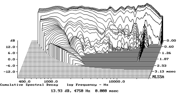
Fig.9 Q Acoustics 5040, cumulative spectral-decay plot on tweeter axis at 50" (0.15ms risetime).
In the time domain, the 5040's step response (fig.8) indicates that the three drive units are connected in positive acoustic polarity. The decay of the tweeter's step, which arrives first at the microphone, blends smoothly with the start of the woofers' step, which implies optimal crossover implementation. The 5040's cumulative spectral-decay plot on the tweeter axis (fig.9) features a clean initial decay. (As always, ignore the apparent low-level ridge of delayed energy just below 16kHz, which is due to interference from the MLSSA host PC's video circuitry.)
Footnote 1: Every time I measure a loudspeaker, I also measure one my 1970s-vintage LS3/5a's to make sure that a systematic error hasn't occurred. Footnote 2: EPDR is the resistive load that gives rise to the same peak dissipation in an amplifier's output devices as the loudspeaker. See "Audio Power Amplifiers for Loudspeaker Loads," JAES, Vol.42 No.9, September 1994, and stereophile.com/reference/707heavy/index.html.