Sidebar 3: Measurements
KR was still working on his review at the time I was scheduled to measure the Merging Hapi MkII, so Independent Audio loaned me a different sample for the testing. This sample had the serial number H95861 and was running firmware version 1.5.1b55774. I followed the instructions in the quick-start guide to download and install both the Merging MTDiscovery app and the RAVENNA/AES67 Virtual Audio Device (VAD) driver on my MacBook Pro. After I connected the Hapi to my router, the app found and identified it and opened its local control webpage on my browser. This page allowed me to select the digital input—AES3 or S/PDIF—set the maximum output level, choose the reconstruction filter, adjust the volume (in accurate 0.5dB steps), and select other functions. All the functions can be operated with the front-panel push knob, but the webpage is easier to use.
I used my Audio Precision SYS2722 system for the measurements, repeating some of the tests with the higher-resolution Audio Precision APx555. My Hapi sample was fitted with the optional DA8P D/A module; this had the serial number DP85778 (Run 14). The multichannel balanced analog output is implemented with a female, Tascam-standard DB-25 jack. I borrowed a two-channel DB-25–XLR adapter cable from KR for the testing. The Hapi's AES3 digital input is implemented with another DB-25 jack. As I didn't have a compatible adapter cable, I used the optical S/PDIF input for the testing, repeating some of the measurements with AES67 network data sourced from Adobe Audition running on my laptop. (There were no differences.)
I used the local webpage to set the Hapi to automatically accept the sample rate of the incoming data. (The rate can also be set manually.) All the testing was performed with the volume control set to its maximum and the maximum gain set to +18dBu. With those settings, a 1kHz digital signal at 0dBFS resulted in an output level of 6.55V. Setting the maximum gain to +24dBu increased the level by 6dB, as expected. The headphone output on the front panel has a fixed maximum level, this measuring 1.266V with a 1kHz tone at 0dBFS. The Hapi preserved absolute polarity, ie, was noninverting, from both the balanced and headphone outputs. The balanced output impedance is specified as a low 90 ohms; I measured 87 ohms from 20Hz to 20kHz. The headphone output impedance was 20 ohms at all audio frequencies.
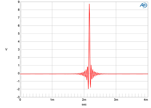
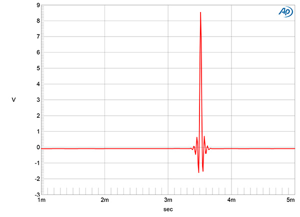
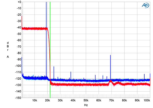
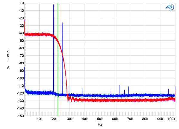
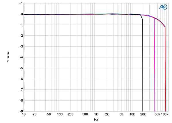
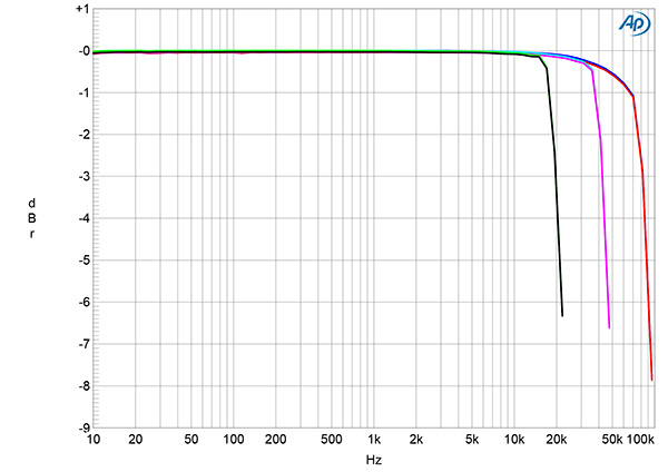
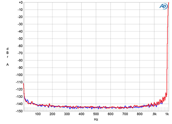
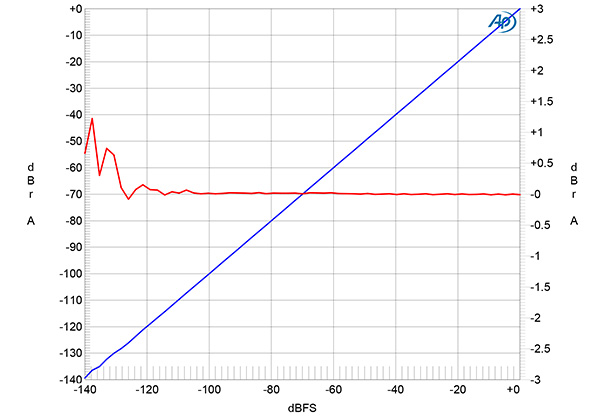
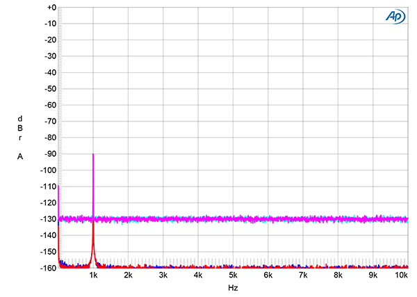
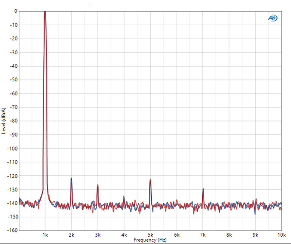
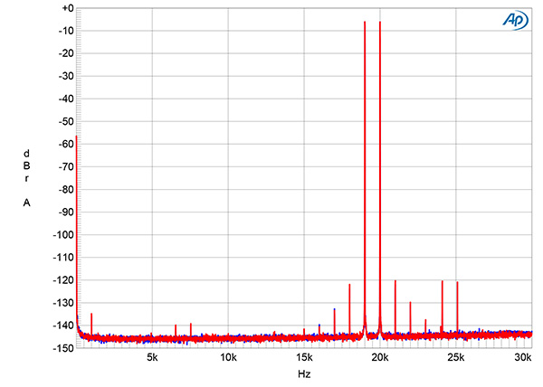
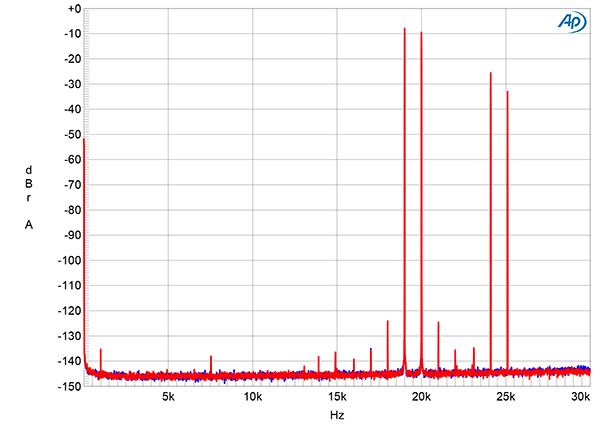
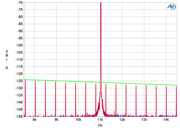
Fig.1 Merging Hapi MkII, Sharp filter, impulse response (one sample at 0dBFS, 44.1kHz sampling, 4ms time window).
Fig.2 Merging Hapi MkII, Slow filter, impulse response (one sample at 0dBFS, 44.1kHz sampling, 4ms time window).
The Hapi offers a choice of four reconstruction filters: Slow, Sharp, Apodizing, and Brickwall. The Sharp filter's impulse response with 44.1kHz data (fig.1) indicates that this is a conventional linear-phase type, with time-symmetrical ringing on either side of the single sample at 0dBFS. The Brickwall and the Apodizing filters' impulse responses were identical to the Sharp filter's. The Slow filter's impulse response (fig.2) shows that this is a very short linear-phase filter, with minimal ringing.
Fig.3 Merging Hapi MkII, Apodizing filter, wideband spectrum of white noise at –4dBFS (left channel red, right magenta) and 19.1kHz tone at 0dBFS (left blue, right cyan), with data sampled at 44.1kHz (20dB/vertical div.).
Fig.4 Merging Hapi MkII, Slow filter, wideband spectrum of white noise at –4dBFS (left channel red, right magenta) and 19.1kHz tone at 0dBFS (left blue, right cyan), with data sampled at 44.1kHz (20dB/vertical div.).
With 44.1kHz-sampled white noise, the Hapi's response with the Apodizing filter rolled off sharply above 20kHz (fig.3, red and magenta traces), reaching full stop-band attenuation at 22.05kHz, half the same rate, as indicated by the vertical green line in this graph. The aliased image at 25kHz of a full-scale tone at 19.1kHz (blue and cyan traces) is suppressed by 100dB, and the highest-level distortion harmonic is the third, at –83dB (0.004%). The Brickwall filter (not shown) behaved identically, other than having a much lower level of the third harmonic. The Sharp filter's output (not shown) reached full stop-band attenuation at 24kHz. The Slow filter's output was down by 3dB at 20kHz and, as expected, its ultrasonic rolloff was the slowest of the four filters (fig.4), with the aliased image at 25kHz suppressed by 28dB.
Fig.5 Merging Hapi MkII, Brickwall filter, frequency response at –12dBFS into 100k ohms with data sampled at: 44.1kHz (left channel green, right gray), 96kHz (left cyan, right magenta), and 192kHz (left blue, right red) (1dB/vertical div.).
Fig.6 Merging Hapi MkII, Slow Filter, frequency response at –12dBFS into 100k ohms with data sampled at: 44.1kHz (left channel green, right gray) and 192kHz (left blue, right red) (1dB/vertical div.).
Fig.7 Merging Hapi MkII, 24-bit data, spectrum, 10Hz–1kHz, with noise and spuriae of dithered, 1kHz tone at 0dBFS (left blue, right red; linear frequency scale) (20dB/vertical div.).
Figs.5 and 6 respectively show the Hapi's frequency response with the Brickwall and Slow filters in greater detail. The sample rates are 44.1kHz (green and gray traces), 96kHz (cyan, magenta traces), and 192kHz (blue, red traces). The Apodizing filter differed from the other filters in having some passband ripple. Channel separation (not shown) was an excellent 113dB in both directions at 1kHz and still 110dB at the top of the audioband. Fig.7 shows the Hapi's low-frequency noisefloor as it drove a full-scale 1kHz tone with the volume control set to its maximum of "0.0dB." The level of the random noise is very low, and no AC supply–related spuriae are present.
Fig.8 Merging Hapi MkII, 1kHz output level vs 24-bit data level in dBFS (blue, 20dB/vertical div.); linearity error (red, 1dB/vertical div.).
Fig.9 Merging Hapi MkII, spectrum with noise and spuriae of dithered 1kHz tone at –90dBFS with 24-bit data (left blue, right red) and 16-bit data (left cyan, right magenta) (20dB/vertical div.).
Fig.10 Merging Hapi MkII, waveform of undithered 1kHz sinewave at –90.31dBFS, 16-bit data (left channel blue, right red).
Fig.11 Merging Hapi MkII, waveform of undithered 1kHz sinewave at –90.31dBFS, 24-bit data (left channel blue, right red).
The red trace in fig.8 plots the error in the analog output level as a 24-bit, 1kHz digital tone stepped down from 0dBFS to –140dBFS. Even at the lowest level, the amplitude error is 1.5dB, which implies very high resolution. When the Hapi decoded dithered 16-bit data representing a 1kHz tone at –90dBFS (fig.9, cyan and magenta traces), the tone was reproduced at the correct level and the noisefloor is that of the LSB-level dither. With dithered 24-bit data (blue, red traces), the noisefloor dropped by 30dB, which suggests the Hapi's DAC module offers a superbly high resolution of 21 bits. With undithered 16-bit data representing a tone at exactly –90.31dBFS (fig.10), the three DC voltage levels described by the data were accurately reproduced. With undithered 24-bit data, the waveform was a clean sinewave, despite the very low signal level (fig.11).
Fig.12 Merging Hapi MkII, 24-bit data, spectrum of 1kHz sinewave, 10Hz–10kHz, at 0dBFS into 200k ohms (left channel blue, right red; linear frequency scale).
The second harmonic was the highest, at just –123dB or 0.00007% (fig.12), with the fifth harmonic slightly lower in level. This graph was taken with the Audio Precision APx555's input impedance set to the high 200k ohms. With the load impedance reduced to the punishing 600 ohms, the third harmonic was now higher in level than the second but still lay at a very low –119dB (0.00011%).
Fig.13 Merging Hapi MkII, Apodizing filter, 24-bit data, HF intermodulation spectrum, DC–30kHz, 19+20kHz at 0dBFS peak, sampled at 44.1kHz.
Fig.14 Merging Hapi MkII, Slow filter, 24-bit data, HF intermodulation spectrum, DC–30kHz, 19+20kHz at 0dBFS peak, sampled at 44.1kHz.
The Hapi's behavior with an equal mix of 19 and 20kHz tones with a peak level of 0dBFS depended on the reconstruction filter. With all the filters, the difference product at 1kHz was vanishingly low in level, at –136dB. With the Sharp and Brickwall filters (fig.13), the higher-order intermodulation products were also very low in level, at less than –120dB. As expected from fig.4, the levels of the aliased images of the two high-frequency tones were much higher with the Slow filter (fig.14), but actual intermodulation products were still very low, even into 600 ohms.
Fig.15 Merging Hapi MkII, high-resolution jitter spectrum of analog output signal, 11.025kHz at –6dBFS, sampled at 44.1kHz with LSB toggled at 229Hz: 16-bit TosLink data (left channel blue, right red). Center frequency of trace, 11.025kHz; frequency range, ±3.5kHz.
Fed with 16-bit Miller-Dunn J-Test data via TosLink, the Hapi featured superb jitter rejection. All the odd-order harmonics of the LSB-level, low-frequency squarewave lay at the correct levels, indicated by the sloping green line in fig.15, and there were no spurious tones present. With 24-bit J-Test data (not shown), the noisefloor was commendably clean.
With its superbly high resolution, vanishingly low levels of noise and distortion, and superb jitter rejection, Merging's Hapi MkII offers state-of-the-digital-art measured performance.—John Atkinson