Editor's Note: The matter of whether—and if so, how—speaker cables and interconnects can affect the sound of an audio system has vexed the audiophile community since Jean Hiraga, Robert Fulton, and others first made us aware of the subject in the mid-1970s. Most of the arguments since then have involved a great deal of heat but not much light. Back in August 1985, Professor Malcolm Omar Hawksford Ph.D (of the UK's University of Essex and a Fellow of the Audio Engineering Society) wrote an article for the British magazine Hi-Fi News & Record Review, of which I was then Editor, in which he examined AC signal transmission from first principles. Among his conclusions was the indication that there is an optimal conductor diameter for audio-signal transmission, something that I imagined might lead to something of a conciliation between the two sides in the debate. Or at least when a skeptic proclaimed that "The Laws of Physics" don't allow for cables to affect audio performance, it could be gently pointed out to him or her that "The Laws of Physics" predict exactly the opposite.
Well, I was wrong. Ten years later, as described in my recent "Wired!!!" essay (June 1995) the "cables make a difference/no they don't" flame war continues unabated (though many of the more sonically successful "audiophile" cables tend to use conductors of the predicted optimal size). I asked Malcolm Omar, therefore, to revise and rewrite his 1985 article for Stereophile. The essential math may look intimidating, but it's not as hard to grasp as it looks (you don't lose points for skipping it). The conclusions are both fascinating and essential reading for anyone who wishes to design audio cables.—John Atkinson
Audiophiles are excited. A special event has occurred that promises to undermine their very foundation and transcend "the event sociological"—a minority group now cite conductor and interconnect performance as a limiting factor within an audio system. The skeptical masses, however, remain content to congregate with their like-minded friends and make jokes in public about the vision of the converted. They are content to watch their distortion-factor meters confidently null at the termination of any old piece of wire (even rusty nails, it seems). Believing in Ohm's Law, they feel strong in their brotherhood—at least that's how it seemed back in 1985.
But the revolution moves forward...
This article examines propagation in cables—especially within conductive material—from the fundamental principles of electromagnetic theory. The aim is to consider mechanisms that form a more rational basis for an objective understanding of claimed sonic anomalies in interconnects, especially as the rumors about single-strand, thin wires persist. Objective understanding relates to the choice of model used to visualize a phenomenon; thus we shall take a theoretic stance and commence with the work of Maxwell. The equations of Maxwell (see sidebar) concisely describe the foundation and principles of electromagnetism; they are central to a proper mathematical modeling of all electromagnetic systems. These equations are presented here in standard differential form and succinctly encapsulate the principles of electromagnetics, although further background can be sought from a wide range of texts (see Sidebar 1). Maxwell's equations support a wave equation that governs the propagation of both the electric and magnetic fields in space and time, where the wave equation describing a propagating electric field E-Bar in a general lossy medium of conductivity σ (sigma), permittivity ε (epsilon) and permeability µ (mu) can be succinctly derived as follows:
Applying the vector operator curl on the Faraday equation,
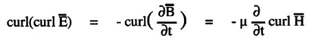 Substituting, B-Bar = µH-Bar and for curl H-Bar from Ampere's law,
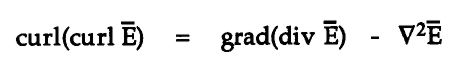
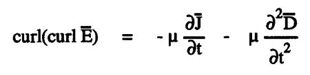 Substituting J-Bar = σ E-Bar , D-Bar = εbE-Bar and using the vector identity,
 The generalized wave equation in a conductive medium then follows as
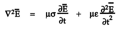 In this equation, ∇2 is the vector Laplace operator, and we have assumed from Gauss's theorem that div bE-Bar = r/ε = 0 for a charge-free region. A similar equation can also be derived in terms of the H-Bar field, where, because of the symmetry of Maxwell's equations,
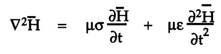 In practice we shall consider only the E-Bar field, as the H-Bar field can be derived from Faraday's law by integrating over time the vector curl E-Bar, which reveals that at every point in space E-Bar and H-Bar are mutually at right angles, and also lie in a plane at right angles to the direction of propagation (fig.1).
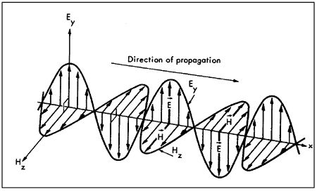 Fig.1 A propagating electromagnetic wave. The sinusoidally varying magnetic field is at right angles to the sinusoidally varying electric field, and both are at right angles to the direction of propagation.
Consider a steady-state, sinusoidal electric field E-Bar propagating within a medium of finite conductivity where, because of the conversion of electrical energy into heat within a conductor, the traveling wave must experience attenuation. This suggests that a steady-state wave of sinusoidal form should decay exponentially as a function of distance z,
E = Eσ–αzsin(ωt – βz)
α (alpha) is defined as the attenuation constant, while the phase of the wave as a function of distance is determined by the phase constant β (beta) = 2Π/λ, where λ (in meters) is the wavelength of the propagating field and ω (omega) = 2Πf, the angular frequency in radians/second.
An exponential decay is a logical choice, as for each unit distance the wave propagates it is attenuated by the same fractional amount. The electric field E is aligned to propagate in a direction z, where the direction of E is at 90° (right-angles) to z as shown in fig.1, where several phases are illustrated. Consequently, at a fixed point of observation z, E varies sinusoidally, while for constant time t, E plotted against z is a sinewave with exponential decay.
To check the validity of this solution, the function for E must satisfy the wave equation. This validation also enables the constants α and β to be expressed as functions of σ, ε, µ, and ω. However, because this substitution, although straightforward, is somewhat tedious, I will show only the initial working and then state the conclusion:
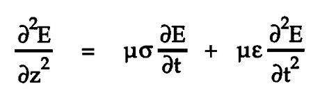
Substitute the assumed solution into the wave equation where, if propagation is assumed to take the direction z,
Fig.1 A propagating electromagnetic wave. The sinusoidally varying magnetic field is at right angles to the sinusoidally varying electric field, and both are at right angles to the direction of propagation.
Consider a steady-state, sinusoidal electric field E-Bar propagating within a medium of finite conductivity where, because of the conversion of electrical energy into heat within a conductor, the traveling wave must experience attenuation. This suggests that a steady-state wave of sinusoidal form should decay exponentially as a function of distance z,
E = Eσ–αzsin(ωt – βz)
α (alpha) is defined as the attenuation constant, while the phase of the wave as a function of distance is determined by the phase constant β (beta) = 2Π/λ, where λ (in meters) is the wavelength of the propagating field and ω (omega) = 2Πf, the angular frequency in radians/second.
An exponential decay is a logical choice, as for each unit distance the wave propagates it is attenuated by the same fractional amount. The electric field E is aligned to propagate in a direction z, where the direction of E is at 90° (right-angles) to z as shown in fig.1, where several phases are illustrated. Consequently, at a fixed point of observation z, E varies sinusoidally, while for constant time t, E plotted against z is a sinewave with exponential decay.
To check the validity of this solution, the function for E must satisfy the wave equation. This validation also enables the constants α and β to be expressed as functions of σ, ε, µ, and ω. However, because this substitution, although straightforward, is somewhat tedious, I will show only the initial working and then state the conclusion:
Substitute the assumed solution into the wave equation where, if propagation is assumed to take the direction z,
 It follows that the function for E is a solution to the wave equation, provided that
β2 – α2 = µεω2
It follows that the function for E is a solution to the wave equation, provided that
β2 – α2 = µεω2
αβ = ωµσ/2 Hence solving for α and β,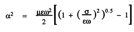 β = ωµσ/2α
where the constants α and β that govern the velocity and attenuation of the propagating field can be expressed in terms of the angular frequency ω and the parameters µ, ε, and σ, which are documented for most materials. (α and β are sometimes expressed as a complex number in terms of the propagation constant γ (gamma), where γ = α + jβ.)
β = ωµσ/2α
where the constants α and β that govern the velocity and attenuation of the propagating field can be expressed in terms of the angular frequency ω and the parameters µ, ε, and σ, which are documented for most materials. (α and β are sometimes expressed as a complex number in terms of the propagation constant γ (gamma), where γ = α + jβ.)
This article examines propagation in cables—especially within conductive material—from the fundamental principles of electromagnetic theory. The aim is to consider mechanisms that form a more rational basis for an objective understanding of claimed sonic anomalies in interconnects, especially as the rumors about single-strand, thin wires persist. Objective understanding relates to the choice of model used to visualize a phenomenon; thus we shall take a theoretic stance and commence with the work of Maxwell. The equations of Maxwell (see sidebar) concisely describe the foundation and principles of electromagnetism; they are central to a proper mathematical modeling of all electromagnetic systems. These equations are presented here in standard differential form and succinctly encapsulate the principles of electromagnetics, although further background can be sought from a wide range of texts (see Sidebar 1). Maxwell's equations support a wave equation that governs the propagation of both the electric and magnetic fields in space and time, where the wave equation describing a propagating electric field E-Bar in a general lossy medium of conductivity σ (sigma), permittivity ε (epsilon) and permeability µ (mu) can be succinctly derived as follows:
Substituting, B-Bar = µH-Bar and for curl H-Bar from Ampere's law,
Substituting J-Bar = σ E-Bar , D-Bar = εbE-Bar and using the vector identity,
The generalized wave equation in a conductive medium then follows as
In this equation, ∇2 is the vector Laplace operator, and we have assumed from Gauss's theorem that div bE-Bar = r/ε = 0 for a charge-free region. A similar equation can also be derived in terms of the H-Bar field, where, because of the symmetry of Maxwell's equations,
In practice we shall consider only the E-Bar field, as the H-Bar field can be derived from Faraday's law by integrating over time the vector curl E-Bar, which reveals that at every point in space E-Bar and H-Bar are mutually at right angles, and also lie in a plane at right angles to the direction of propagation (fig.1).
Fig.1 A propagating electromagnetic wave. The sinusoidally varying magnetic field is at right angles to the sinusoidally varying electric field, and both are at right angles to the direction of propagation.
It follows that the function for E is a solution to the wave equation, provided that
αβ = ωµσ/2 Hence solving for α and β,
β = ωµσ/2α
where the constants α and β that govern the velocity and attenuation of the propagating field can be expressed in terms of the angular frequency ω and the parameters µ, ε, and σ, which are documented for most materials. (α and β are sometimes expressed as a complex number in terms of the propagation constant γ (gamma), where γ = α + jβ.)