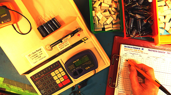
Testing capacitors at Ben Duncan Research using high-speed production component testers, made in England by Wayne-Kerr (1980s) and Peak (2010s). Parts are numbered and seven performance parameters that can affect sonics like loss at 10kHz, are manually tabulated. Rogue parts can be quickly identified by eye and relieved of musical duties. Photo: Ben Duncan.
Have you ever suspected that the component you bought after diligent research is somehow not "typical"? That its sound seems to bear little resemblance to the descriptions in the reviews you read? Sure, you listened to the unit before purchase, but the one you took out of the box at home—was that the same unit? And if you suspect your new unit's sonic quality is below par, just how do you or your dealer go about proving it?
The inanimate world [1] created by mankind has as many foibles as the humans it delights in playing tricks on. Over a century ago, the English zoologist T.H. Huxley wrote, "The known is finite, the unknown infinite; intellectually we stand in an islet in...an illimitable ocean of inexplicability. Our business...is to reclaim a little more land." In this article, I will try to clear some of the mud off a few square yards, homing in on the meaning of some manufacturing variations that occur in even the finest music-replay systems.
Like racing engines, the best hi-fi systems are finely tuned—meaning the end result depends on many fine details. A small variation in just one of these details can cause an unexpectedly large loss of performance. Engines and sound systems are both built from many component parts, often thousands—depending where you draw the line. Readers involved in any kind of engineering will be aware that every manufactured artifact differs slightly from the next. The range of differences between manufactured, ideally uniform objects is called tolerance. Awareness of tolerance—ie, sameness—hinges on the ability to measure and resolve fine differences. Metal can be cut, cast, or ground to tolerances of fractions of a millimeter—equivalent to tolerances better than, say, 0.01% for enclosures and heatsinks. Wood can't be measured meaningfully so finely, because it contracts and expands much more, and more readily, than metal, depending on temperature, humidity, and how long it has been seasoned. Capacitors and resistors—the wood and metal of electronics—are commonly made to comparatively loose tolerances of ±1, 2, 5, or 10%. Although the best equipment uses tighter resistor tolerances, up to 0.1%, capacitor tolerances tighter than 1% are rare and troublesome. The parameters of active devices (ie, bipolar transistors, FETs, tubes, op-amps, and diodes) are held within ±5% at best and can be as broad as ±70%, depending on cost, measurement temperature, design and manufacturing finesse, and the attribute in question. Transducer tolerances are as "loose" as active devices. If an object has only one critical parameter (a measurable quality or attribute), then the manufacturer can simply decide on the acceptable variation or difference, pick any samples that fall within this range, and reject any that don't. If 20% of the objects pass this test, then 80% will be rejects.
To illustrate the effect of component tolerances on the simplest level, I entered a model of a minimal LP-replay system into MicroCAP III, a PC-based circuit simulator (footnote 1). Looking at the block schematic (fig.1), the model comprises a cartridge (only the electrical internals are modeled), a cable, and a phono amp headed by a discrete buffer, followed by the RIAA EQ circuit, which uses two op-amps modeled on the ubiquitous NE5534 chip.
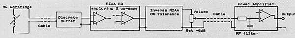
Fig.1 Block schematic of the minimum disc replay path, used to analyze individual systems' frequency-response variations.
To simulate the effect of the RIAA pre-emphasis present on the disc, I have followed the preamp's RIAA stage with a reference inverse RIAA circuit. (This was set to have perfect, zero tolerance in the simulation, so it plays no part in any variations.) There follows a volume control set 6dB below maximum, more cable, and a power amplifier with a typical voltage gain of x28, or just under 26dB. To make the simulation practicable, the last stage was simplified to be a power op-amp (footnote 2).
The full circuit contains a large number of parts, each with tolerances typical of mid- to high-end equipment, ranging from ±1% for resistors, up to ±60% for the looser active-device parameters (like Hfe, representing a transistor's raw gain), and ±70% for cable parameters—allowing, within reason, for the different lengths used in real systems. As well as its value, in Ohms, Farads, or Henries, each passive component in the model has the tolerance of this quantity in ±% noted, and the temperature coefficient in ppm (parts per million). Other than the simplifications noted, the model neglects long-term component value changes occurring over time, or one-off changes caused during manufacture by soldering and testing.
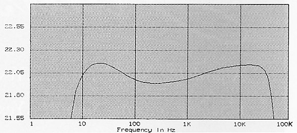
Fig.2 Predicted circuit frequency-response assuming zero tolerance (0.25dB/vertical div.).
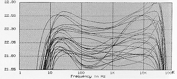
Fig.3 Predicted frequency-response variation in 25 randomly selected systems (0.25dB/vertical div.).
Footnote 1: Before the advent of circuit simulation in the mid-'70s, tolerance analysis for any system containing hundreds of variables was too tedious to perform without teams of mathematicians, and not justifiable outside of critical space and military equipment. Instead, makers flew by the seats of their pants, and problems caused by out-of-tolerance (but in-spec) parts were usually only discovered by production tests or in the field, somewhat after the stable door had been bolted. Footnote 2: To save enough memory to make the simulation possible on a PC-XT, the op-amp model behaves like an amplifier, but greatly reduces the number of nodes in the SPARSE matrix. The speaker cables' and drive-unit's electrical portions are excluded for the same reason. Even with all these simplifications, total parts count is around 200.