
Tutorial: Understanding Noise And Signal Plots
The sounds we hear are rarely one thing, in fact sounds convey meaning by changing and combine tonal and atonal elements. Nevertheless engineers will spend a lot of effort using tones (single notes) to investigate frequency response and non-linearity. Similarly we measure noise to try to understand how much there is. In our world background noise is an irremovable feature. A recording system adds noise as do distribution and replay systems. If we are to design or specify or compare, we need a framework within which to be able to estimate the significance of measurements of different sounds and signals.
Human hearing has at least six nonlinearities that should be taken into account when we evaluate the properties of music signals or reproduction systems, these are threshold, compression, selectivity, response to sound envelope, object externalisation and context (including memory).
Some of these are simpler than others to predict but let's just look at how we can decide the equivalence between tonal signals and noise.
The human hearing system features frequency selectivity which (in the steady state) can be thought of as an array of approximately 3500 filters whose bandwidth depends on the centre frequency and level; it is most selective for quiet sounds. Although the neural system is capable of extracting a huge amount of information from this filter bank, at the energy level, sounds that are close together in frequency accumulate intensity that can lead to detection or to an impression of loudness. So if we are presented with a wideband noise our hearing will broadly accumulate intensity within each band of noise or signals or both. To correctly estimate the audibility of a noise or the threshold of a tone in noise, knowing this bandwidth in context is essential.[12]
 To map a noise signal to its effective loudness so we can compare it with a tone. The wider the bandwidth the more a noise will accumulate intensity—see Figure 2.
To map a tonal threshold so we can compare it to a noise—see Figure 3. [12][14].
To map a noise signal to its effective loudness so we can compare it with a tone. The wider the bandwidth the more a noise will accumulate intensity—see Figure 2.
To map a tonal threshold so we can compare it to a noise—see Figure 3. [12][14].
 For those interested we strongly recommend reading and absorbing the concepts covered in [1] which is only two pages long but covers a lot of ground. The most important points being made relate to temporal dispersion of signals between the performance and listener and rooting the targets in the analogue, not digital domain. The paper Stuart and Craven presented to AES in 2014 goes much deeper into the 'why' but takes more effort to grasp! [2]
Let's do another tutorial:
For those interested we strongly recommend reading and absorbing the concepts covered in [1] which is only two pages long but covers a lot of ground. The most important points being made relate to temporal dispersion of signals between the performance and listener and rooting the targets in the analogue, not digital domain. The paper Stuart and Craven presented to AES in 2014 goes much deeper into the 'why' but takes more effort to grasp! [2]
Let's do another tutorial:
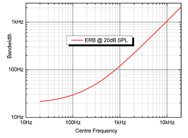
Figure 1: Showing ERB—the noise bandwidth of human hearing as a function of frequency when the intensity of the local stimulus is 20dB SPL. Above 300Hz the relationship is almost logarithmic which is why proportional-bandwidth measures such as 1/3 octave can be helpful. In fact 1/8 octave is the closer fit over the sensitive range.
Figure 1 shows a plot of ERB, the equivalent rectangular noise bandwidth for signal at 20dB SPL. We can use this information in two ways:
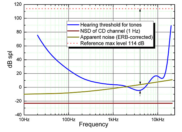
Figure 2: The blue curve shows the threshold for detection of pure tones (often called the threshold of hearing). In this case the curve plotted is for free-field listening within an arc of ±30°. Overlaid on this is the noise-floor of a CD channel (44.1kHz 16-bit sampling using TPDF dither) with a very high acoustic gain (in this case a full-scale signal would give 114dB SPL. As shown earlier, the NSD for this channel is 137dB below 114, ie, at –23dB SPL/√Hz. The audible significance of this noise is estimated using ERB correction and is shown as the olive plot. Detectability is a very complex topic but where sound components using this measure reach the blue line there is a possibility of detection that increases as the signal estimate increases further (above the blue line).[12] Note that this plot suggests we will hear the noise at this volume setting and it will manifest between 2 and 8kHz. At 4kHz this curve is around 110dB below full scale (see arrow) and a tone at this level would be audible if the room is sufficiently quiet. This is a graphical explanation of how we can hear some isolated signals below the LSB (notionally –93dBFS in a 16-bit PCM channel). Of course, channels exploiting noise-shaping can reduce the impact of dither and quantisation noise.
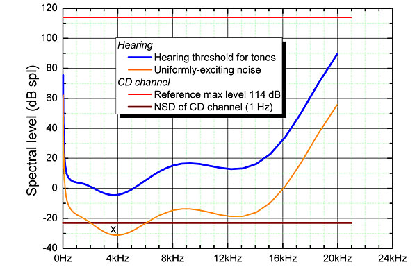
The visualisation in Figure 2 helps to estimate audibility but for a coding system we need to see the information content more clearly. We can estimate the information content in a signal by examining the area it projects onto a Shannon diagram and in these cases it is useful to not weight measurements of noise according to human psychoacoustics but rather to remap the human hearing-threshold for tones onto a uniformly exciting-noise at threshold. This noise has the shape shown in the orange curve in Figure 3 and has the very interesting property that if we gradually increase such a noise in level from below audibility, at a certain point (plotted on the graph), unlike white noise, it will become detectable at all frequencies simultaneously.
Figure 3: Showing the use of threshold-equivalent UENTH to estimate the significance of shaped or wide-band noise in a Shannon diagram. Here we can see if a noise spectrum might be audible, but unlike in Figure 2, we cannot determine the detectability of a tone without interpreting both curves.[12][14]
Temporal Precision
There is misunderstanding of temporal accuracy in a digital channel. In our communications we refer to 'blur', but commentators tend to think we are discussing timebase. Here's a typical one:
Time resolution in digital is infinite!
A major failing of audio systems is that there is no clear end-to-end specification. We can have individual components or parts of the chain with wide bandwidth or low noise, but the final result depends on the narrowest part of the pipe. This is one reason there has been so much confusion around high-sample-rate audio—there is less point in 192kHz sampling if the amplifier stops at 20kHz.