Reference

A block diagram of the Trifield circuit is shown in fig.1. First, the left and right channels are passed through an MS matrix to convert them into sum (M) and difference (S) signals. In the Bell-Klipsch scheme, the M component was fed directly to the center speaker, with appropriate gain correction, whereas here it is first divided into two overlapping frequency ranges by complementary low-pass and high-pass filters, their corner frequencies set at 5kHz or above. (Gerzon's listening tests showed that the exact corner frequency and the filters' rate of rolloff were uncritical, although the transition should not be too rapid.) Each filtered signal then passes to a sine/cosine potential divider, which is set differently for each frequency band. Only with this arrangement, Gerzon found, could a wide stereo image and sharpened central focus be traded off effectively against one another across the entire audible spectrum.

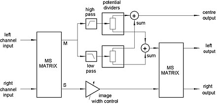Fig.1 The Trifield circuit.

The outputs of the potential dividers are then summed as shown, one sum being fed to the center speaker and the other to a second MS matrix, where, in combination with the difference (S) signal from the input matrix, feeds for the left and right speakers are reconstructed. A variable attenuator in the S line provides a stereo width control; otherwise, the difference signal is unaltered in its passage through the circuit, provided that the crossover filters in the M path introduce no phase distortion—something that is easily achievable today with digital filters. If the filters are not linear-phase, then an all-pass network has to be added to the S path, to mimic their phase behavior.

In the consensus view of audio reviewers worldwide, Trifield really is capable of delivering on its promise to enhance and stabilize the stereo image, and can achieve this with most source material, however it was recorded. There are occasional recordings that don't respond as well to its ministrations, but these are the exception rather than the rule, not least because Trifield makes no assumption about how a recording was made. Instead, it addresses the psychoacoustics of how stereo images are perceived.

Despite this critical acclaim, Trifield—like Ambisonics before it—has never achieved critical mass. Meridian was an early adopter of Trifield in its surround processors and remains faithful to this day, but few others followed Meridian's lead—although for a while Yamaha did offer Trifield in its home-theater products.

Belatedly, the audio industry has now begun to catch up—not by adopting Trifield, but by developing alternatives. Some of these new algorithms, like Trifield, concern themselves solely with the task of improving the stereo image through the addition of further speakers arrayed between the normal stereo pair (footnote 7). More often, the aim is to upmix two-channel stereo signals to five channels suitable for replay over a conventional 5.1-channel speaker array. So in addition to generating a center channel, these algorithms also work to create surround channels. In this respect they are successors to the simple ambience-extraction techniques first developed in the early 1970s—which begins the second strand of our story.

Behind You
An odd thing happened in the August 1970 issue of British hi-fi magazine Hi-Fi News: the publication of two pioneering articles on the subject of ambience extraction by authors who had been working on it independently. One was Michael Gerzon again (footnote 8), taking his first steps on the path that would lead to Ambisonics; the other, more famously, was David Hafler, whose name has been associated ever since with this most basic of ambience-extraction processes.

Although they had worked along similar lines, what Gerzon and Hafler did was not identical. Gerzon, still a student at Oxford at the time, originally used a four-speaker layout (fig.2), with one speaker firing straight ahead and carrying the sum of the two channels (L+R); two at either side carrying the left- and right-channel signals, respectively; and the last at the rear, carrying the L–R difference signal. Gerzon also suggested the alternative speaker layout of fig.3, in which each speaker carries a particular combination of the left and right channels. Hafler suggested the alternative speaker layout shown in fig.4, which retains the conventional stereo disposition of the left and right speakers, but adds a center front speaker that carries the sum signal, and a center rear speaker that carries the difference signal. In a follow-up article a year later, Gerzon built on these ideas and suggested some enhancements (footnote 9).

Fig.2 Gerzon's four-speaker layout.

Fig.3 Gerzon's alternative four-speaker layout.

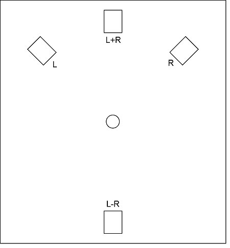Fig.4 Hafler's four-speaker layout.

Gerzon's and Hafler's attempts to extract ambience from a stereo signal and present it behind the listener were both predicated on the assumption that this ambience is present in the L–R difference signal. With some recordings this is sufficiently true for the Hafler system (I'll follow accepted terminology and call it that) to give good results. But as anyone who has tried it knows, this form of ambience extraction gives far from universally positive results—for reasons that are simple enough to identify.

Consider the case of a single sound source that is hard left in the stereo soundstage and so appears only in the left channel. The sum signal (L+R) is then equal to L, as is the difference signal (L–R). So the same signal appears in three speakers: center, left, and rear. Now consider a single sound source that is hard right and so appears in only the right channel. Again, the same signal appears in three speakers—center, right, and rear—but now the rear speaker carries it in antiphase (because L–R = –R). This illustrates how signals that should be confined to the front speakers appear in the rear "ambience" speaker.

There are ways to ameliorate these effects, including the application of delay to the L–R difference signal, whereby the precedence effect ensures that the stereo image remains forward of the listener. But clearly the Hafler system is not a sufficiently clever way to extract ambience from two-channel stereo signals; nor, as we have already seen, is it an optimum way of creating a center channel. With the refinements suggested by Gerzon, it was about the best that could be done in the early 1970s, but today's burgeoning DSP power facilitates more sophisticated approaches.

What is required, clearly, is a method of extracting ambience that adapts itself to the nature of the stereo signal. This prospect will likely send a chill up the spines of those who remember the effect of variable-matrix approaches on matrixed quadraphonic systems, but again, this harks back to a technology that was crude compared to what can be achieved today.

The first step is to divide the signal into short frames and analyze each of them to determine how best to process the signal at that point (footnote 10). One approach to this is to construct an XY or Lissajous graph in which the instantaneous amplitude of one channel (usually the left) is plotted on the vertical axis, and that of the other channel on the horizontal axis. If the two channels carry exactly the same signal, with the same amplitude and phase, then the result will be a straight line at 45° to the horizontal, running bottom left to top right.

Fig.5 shows a typical such graph for a stereo music signal, in this case for an image position to the left of center, so that the angle of the plot is steeper than 45°. This was not culled from a commercial recording but obtained by using the MicSimulator software utility (available from the freeware page on my website, www.audiosignal.co.uk/freeware), which simulates various stereo microphone techniques using monophonic anechoic recordings as source material. The mike technique chosen in this case was a Blumlein crossed pair, which results in pure intensity stereo, where the position of the sound source is represented solely by the relative amplitude of the signal in each channel. From the output WAV file I selected for analysis that section equivalent to an image position of 30° left. Had the output of MicSimulator been used directly, then the resulting XY graph would be a thin, straight line. But I added artificial stereo reverberation (using Adobe Audition) prior to generating the XY graph, which better represents what would be obtained in a normal, live recording environment. As a result, the line has been expanded into something more like an ellipse, the major (ie, long) axis of which is aligned in the same direction.

Fig.5 Lissajous plot for a simulated crossed-pair recording of a single instrument.

By identifying the alignment of this major axis and modifying the difference signal accordingly, we can do much better at extracting the ambience information than we would using the Hafler technique. Instead of taking L–R to be the ambience signal, we first note that, ignoring the ambience component, L is equal to 3.732R in this example (footnote 11)—something we can determine from the angle of the major axis. So by using L–3.732R instead of L–R, we should eliminate the direct signal and extract the ambience alone.

I have considered a very simple case here, of course, with a single sound source, whereas in most recordings multiple sound sources are present at any one time. But so long as these give rise to an XY plot with a clear major axis, this method of ambience extraction gives improved results. The problems come when the XY plot has no clear alignment, such as when noncoincident microphone techniques are used. In such cases, the spacing of the microphones gives rise to a frequency-dependent phase relationship between the two channels, which results in an XY plot whose distribution looks random. Fig.6 illustrates this using the same source signal and angle as in fig.5, but this time with MicSimulator simulating the effect of spaced omnidirectional microphones. As you can see, the plot has no clear alignment.

Fig.6 As fig.5, but this time for a simulated spaced-omni recording.

To overcome this problem, we need to align the left and right channels in such a way as to take account of the time delay between them. In this example, the time delay is about 2.9 milliseconds (equivalent to 128 samples at 44.1kHz); if we offset the left channel by this amount relative to the right channel before generating the XY graph, we achieve the result shown in fig.7. The plot now looks rather more like fig.5—although the alignment of the major axis is shifted because there is much less amplitude difference between the two channels with this recording technique—and we can apply the same approach to extracting the ambience component.

Fig.7 Result of first time-aligning the two channels of fig.6.

Once again, this is a very straightforward case that sidesteps the fact that in most spaced-omni recordings there will be multiple sound sources with different time delays. Nonetheless, statistical comparison of the two channels can be used to identify an optimum time delay for the extraction of the ambience signal.

Does it work?
These examples only scratch the surface of how modern upsampling algorithms are improving on the Hafler technique, but they give a flavor of the methods being used. The key question is: How successful are these new methods? For the moment, we have only the findings of academic listening tests to go by, but it is beginning to look as if a corner may have been turned in this endeavor.

When, in 1998, Francis Rumsey reported controlled listening tests on a selection of upmixing algorithms,12 he found that "in general the front image quality is reduced and the spatial impression slightly improved by processing, and that expert listeners tend to prefer unprocessed material to that which has been processed." In contrast to this, results achieved with a more recent design of algorithm indicate the opposite conclusion,13 although this may relate to the simplicity of the chosen test material. In another significant development, the respected Fraunhofer-Institut in Germany has just released its own upmixing algorithm, SX Pro (the SX stands for Stereo eXtended), which it describes as being based on "a semantic analysis of the input signal that guarantees a high degree of control over the resulting sound image."

Of course, we should be skeptical until we have heard these algorithms working within the context of the highest-quality audio systems, but it may be that the benefits of upmixing two-channel material to five channels at long last outweigh the downsides. For a quest whose origins can be traced back almost 75 years, it's about time.

---

Footnote 7: C. Faller, "Multiple-Loudspeaker Playback of Stereo Signal," JAES, Vol.54 No.11, November 2006 (available from www.aes.org).

Footnote 8: M.A. Gerzon, "Surround Sound from 2-Channel Stereo," Hi-Fi News, August 1970 (downloadable from the Gerzon Archive on my website).

Footnote 9: M.A. Gerzon, "A Year of Surround Sound," Hi-Fi News, August 1971 (downloadable from the Gerzon Archive on my website).

Footnote 10: I believe such time-slicing lies at the core of Dave Griesinger's active steering algorithm, commercially realized in Lexicon's "Logic 7" process.—John Atkinson

Footnote 11: Because the sound source is 30° to the left of center, it is 15° off-axis to the left-channel microphone and 75° off-axis to the right-channel microphone. With figure-8 velocity microphones, the relative levels in the left and right channels are therefore proportional to cos(15)=0.9659 and cos(75)=0.2588, respectively. The ratio of these two figures is 3.732.

Footnote 12: F. Rumsey, "Controlled Subjective Assessments of 2-to-5-Channel Surround Sound Processing Algorithms," Preprint 4654, 104th Audio Engineering Society Convention, May 1998 (available from www.aes.org).

Footnote 13: J. Usher, "A New Upmixer for Enhancement of Reverberance Imagery in Multichannel Loudspeaker Audio Scenes," Preprint 6965, 121st Audio Engineering Society Convention, October 2006 (available from www.aes.org).