Measurements, from January 2022 (Vol.45 No.1):
When Herb Reichert reviewed the Mola Mola Tambaqui in his December 2021 Gramophone Dreams column, he very much liked what he heard from this Bruno Putzeys–designed D/A processor. "During my first days of listening, the Mola Mola's most conspicuous sonic trait was a bright, evenly illumined clarity," he wrote, adding, "Mola Mola's Tambaqui did not whisper—it declared loudly: 'See! The truth is more beautiful than you thought it would be!'" Herb concluded that with the Mola Mola Tambaqui, "Putzeys seems to be punching away at the fundamentals of digital conversion."
After he had written his column, Herb emailed me to suggest that I measure the Tambaqui. I didn't need to be asked more than once.
I controlled the Tambaqui with the MOLAREMOTE app for iOS, which I found straightforward to use, and I used my Audio Precision SYS2722 analyzer to examine the Mola Mola Tambaqui's performance using its TosLink, AES3, and USB inputs. I then repeated some of the tests with the magazine's higher-resolution Audio Precision APx500 analyzer.
The Tambaqui's AES3 and optical and coaxial S/PDIF inputs locked to data sampled up to 192kHz. Apple's AudioMIDI utility revealed that the USB inputs accepted 24-bit integer data sampled at rates up to 768kHz. Apple's USB Prober utility identified the Mola Mola as "MolaMola USB Audio 2.0" from "MolaMola," and the USB port operated in the optimal isochronous asynchronous mode.
The Tambaqui got warm in use, the top panel's temperature stabilizing at 103.8°F (39.9°C). The outputs all preserved absolute polarity, and the output level depended on the gain setting, described in the app as "6V," "2V," or "600mV." A 1kHz digital signal at 0dBFS resulted in levels of 6.11V, 1.93V, or 611mV at the main balanced output, 6.04V, 1.91V, or 604mV at the headphone outputs. The output impedance was 44 ohms at the main balanced outputs and a low 0.47 ohm at the headphone outputs, both values as specified and consistent across the audioband.


The Mola Mola Tambaqui offers state-of-the-digital-art measured performance. I am not surprised HR liked its sound.—John Atkinson
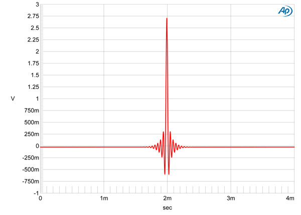
Fig.1 Mola Mola Tambaqui, impulse response (one sample at 0dBFS, 44.1kHz sampling, 4ms time window).
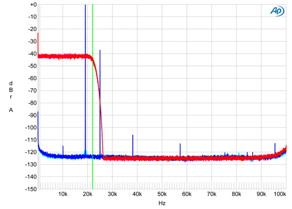
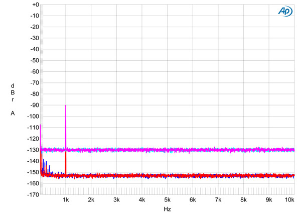
Fig.2 Mola Mola Tambaqui, wideband spectrum of white noise at –4dBFS (left channel red, right magenta) and 19.1kHz tone at 0dBFS (left blue, right cyan), with data sampled at 44.1kHz (20dB/vertical div.).
Fig.3 Mola Mola Tambaqui, frequency response at –12dBFS into 100k ohms with data sampled at: 44.1kHz (left channel blue, right gray), 96kHz (left channel cyan, right magenta), 192kHz (left green, right red) (1dB/vertical div.).
The impulse response with 44.1kHz data (fig.1) indicates that the single reconstruction filter is a conventional linear-phase type, with time-symmetrical ringing on either side of the single sample at 0dBFS. With 44.1kHz-sampled white noise (fig.2, red and magenta traces), the reconstruction filter's response rolled off above 20kHz, reaching full stop-band suppression at 26kHz, a little above half the sample rate (vertical green line). The aliased image at 25kHz of a 19.1kHz tone at 0dBFS (blue and cyan traces) was suppressed by 38dB, and the highest-level distortion harmonic of the 19.1kHz tone, the second, lay at –107dB (0.0004%). The frequency response was flat in the audioband, with then a rolloff that started below half of each sample rate (fig.3). Channel matching was superb.
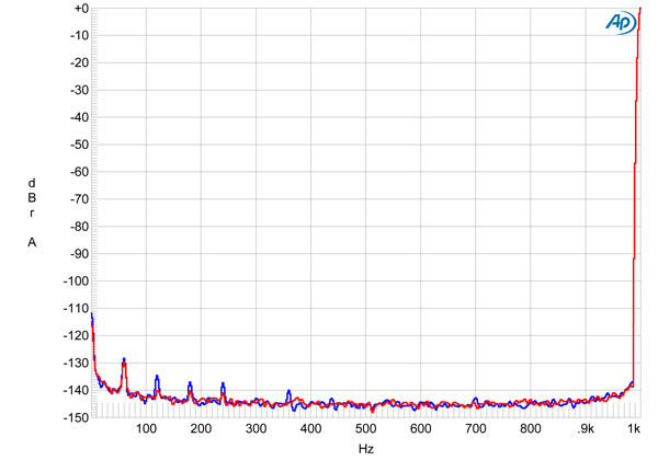
Fig.4 Mola Mola Tambaqui, 2V fixed output, spectrum with noise and spuriae of dithered 1kHz tone at 0dBFS with 24-bit data (left channel blue, right red) (20dB/vertical div.).
Channel separation was 112dB in both directions across the audioband, and the Tambaqui's noisefloor was very low in level (fig.4). This spectrum was taken with the processor's maximum output set to 2V—HR had used the Tambaqui set to 2V maximum output level—and any supply-related spuriae were at –130dB or lower.
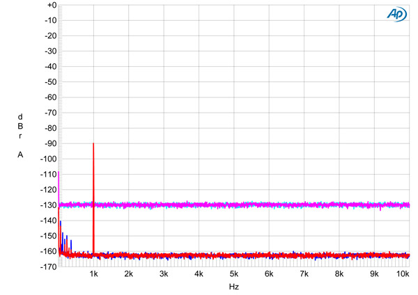
Fig.5 Mola Mola Tambaqui, 6V fixed output, spectrum with noise and spuriae of dithered 1kHz tone at –90dBFS with: 16-bit data (left channel cyan, right magenta), 24-bit data (left blue, right red) (20dB/vertical div.).
Fig.6 Mola Mola Tambaqui, 2V fixed output, spectrum with noise and spuriae of dithered 1kHz tone at –90dBFS with: 16-bit data (left channel cyan, right magenta), 24-bit data (left blue, right red) (20dB/vertical div.).
To examine the Mola Mola's ultimate resolution, I set the maximum output level to 6V and examined the output spectrum with a dithered 1kHz tone at –90dBFS with 16- and 24-bit data (fig.5). With 24-bit data, the noisefloor dropped by 33dB, which implies that the Tambaqui offers almost 22 bits of resolution, the highest I have encountered. Repeating the measurement with the maximum output set to 2V, the increase in bit depth dropped the noisefloor by 24dB (fig.6), which is still 20 bits' worth of resolution.
Fig.7 Mola Mola Tambaqui, waveform of undithered 1kHz sinewave at –90.31dBFS, 16-bit data (left channel blue, right red).
Fig.8 Mola Mola Tambaqui, waveform of undithered 1kHz sinewave at –90.31dBFS, 24-bit data (left channel blue, right red).
With undithered data representing a tone at exactly –90.31dBFS (fig.7), the three DC voltage levels described by the data were well resolved, the ringing of the reconstruction filter could clearly be seen, and DC offset was negligible. With undithered 24-bit data (fig.8), the result was a clean sinewave despite the very low signal level.
Fig.9 Mola Mola Tambaqui, 6V fixed output, spectrum of 1kHz sinewave, DC–10kHz, at 0dBFS into 200k ohms (left channel blue, right red; linear frequency scale).
As implied by the spectrum in fig.2, the Tambaqui featured very low levels of harmonic distortion. I therefore looked at the spectrum of the balanced output with the APx500 analyzer while the processor reproduced a 1kHz tone at 0dBFS (fig.9). Even with the Tambaqui's maximum output level set to 6V, the only harmonic visible was the third, at a roots-of-the-universe level of –130dB (0.00003%).
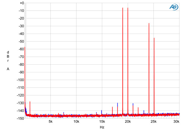
Fig.10 Mola Mola Tambaqui, 2V fixed output, HF intermodulation spectrum, DC–30kHz, 19+20kHz at 0dBFS peak (left channel blue, right red; linear frequency scale).
Intermodulation distortion was also extremely low, even into 600 ohms (fig.10), though moderate-level aliased images of the two high-frequency tones can be seen at 24.1kHz and 25.1kHz.
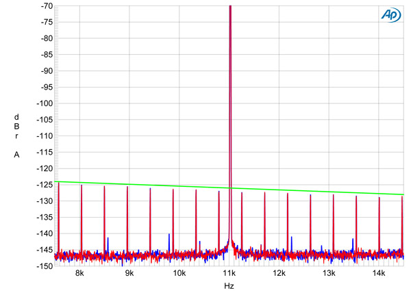
Fig.11 Mola Mola Tambaqui, high-resolution jitter spectrum of analog output signal, 11.025kHz at –6dBFS, sampled at 44.1kHz with LSB toggled at 229Hz: 16-bit TosLink data (left channel blue, right red). Center frequency of trace, 11.025kHz; frequency range, ±3.5kHz.
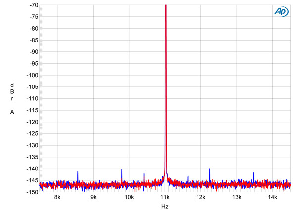
Fig.12 Mola Mola Tambaqui, high-resolution jitter spectrum of analog output signal, 11.025kHz at –6dBFS, sampled at 44.1kHz with LSB toggled at 229Hz: 24-bit TosLink data (left channel blue, right red). Center frequency of trace, 11.025kHz; frequency range, ±3.5kHz.
Tested for rejection of word-clock jitter via its TosLink input, using 16-bit J-Test data sampled at 44.1kHz, the Tambaqui's output was clean. All the odd-order harmonics of the J-Test signal's LSB-level, low-frequency squarewave were very close to the correct levels (fig.11, sloping green line). No supply-related sidebands can be seen, and the random noisefloor is very low in level. However, some very low-level sidebands of unknown origin are visible in the left channel (blue trace). Repeating the test with 24-bit data gave a superb result (fig.12). The left channel's sidebands are still present; at –140dB, however, these are inconsequential.