| Columns Retired Columns & Blogs |
InnerFidelity Headphone Measurements Explained
This story originally appeared at InnerFidelity.com
Udauda's (Rin Choi) Head-Fi Listing of all sites providing headphone measurements, which, unfortunately, doesn't include a link to Marv's measurements at the very bottom of Changstar's home page or the wealth of information in their measurement forum area.
Jude Mansilla (Head-Fi Founder) comments on headphone measurement systems.
Headphone measurements are complicated and relatively difficult to interpret. The following is written to help you understand InnerFidelity's headphone measurements, which can be found here.
Frequency Response
Understanding the Problem
Headphone frequency response measurements are not only difficult to make, but also quite difficult to interpret. Headphones can't be measured with normal measurement microphones, they have to be measured like they are used—coupled to a microphone that mimics the acoustic characteristics of the ear. Essentially, when we measure a headphone, we are taking a measurement of what the ear drum hears.
The problem is, by the time outside sound gets to your ear drum it's not flat any more. Our brain is used to hearing sound with this non-flat ear drum response. When we measure headphones we have to know very precisely what that non-flat ear drum response is so that it can be subtracted from headphone measurements to return them to a flat line for evaluation. In order to understand headphone measurements, you have to understand the various factors considered to develop this headphone target response compensation curve. You'll also have to understand that an industry-wide standardized curve currently doesn't exist (though one is in development), so there is no clear answer regarding "what flat is" with headphones. With this article I hope to provide you with a few helpful concepts and hints, but plenty of questions will remain at the end.
This article will be in two parts. This first part, will explore the target response curve and how to recognize it. The second article will look at specific types of artifacts seen in headphone frequency response measurements, and what they mean.
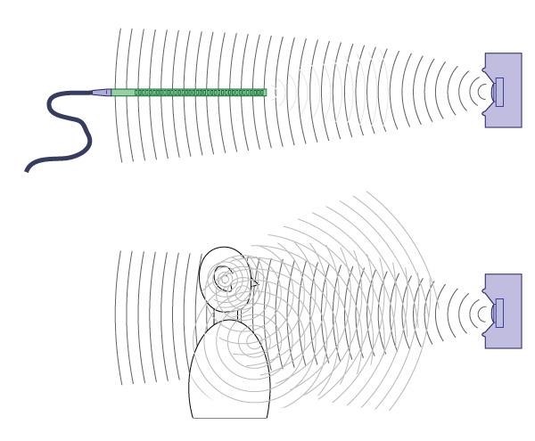
What our ear drum hears in front of a speaker.
At the top of the diagram above, we see a measurement microphone in front of a speaker. Let's assume it's a perfectly flat speaker being measured in an anechoic chamber (a room with no acoustic reflections). The microphone will have a very small interaction with the acoustic energy, but for the most part it is designed to measure very accurately the sound field present without disturbing it. In this case, if the speaker is "flat" (acoustically neutral), the output from the mic will also be flat.
Now, let's remove the mic and put a person in front of the same speaker and look at the signal at that person's ear drum. It will no longer be flat because of a number of acoustic interactions between various parts of the body with the incoming acoustic signal. The graph below shows the various acoustic gain contributors to the frequency shaping heard by a person positioned in front of a speaker.
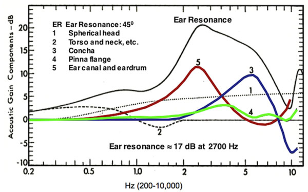
The dotted black line (1) shows the boundary gain from your head. Assume for a moment your head is roughly a one foot sphere. At very low frequencies, with half wavelengths much longer than the dimension of your head, there will be little interaction between the acoustic wave and your head. But as you raise the frequency of the sound to the point where its half-wavelength is of similar dimension as the head, you begin impede the sound and create some gain at the boundary. In the case of a 12" head and the speed of sound at 1126 feet/sec, sound will start getting some gain at around 563Hz. As you can see, the plot of spherical head gain is at 0dB below 300Hz, and then slowly transitions to about +3dB at around 1200Hz. (To the best of my understanding, boundary gain at the side of the head should only be able to deliver 3dB of increase, while the chart shows around 6dB at 10kHz. Sorry, I can't explain why this is so.)
Likewise, your torso (shoulders, chest, belly) will provide some boundary gain. Your body is bigger than your head, so its effect will begin at lower frequencies. But because your ears are not directly attached to your body and are separated at a distance, as soon as the half-wavelength becomes equal to that distance you will begin to lose coupling and the effect will diminish. You can see that dashed line (2) in the chart above indicating the torso providing some gain at lower frequencies to about 1kHz. Between 1kHz and 2kHz this torso curve actually goes negative due to destructive interference between the direct sound at the ear and the sound being reflected off the torso. Above 2kHz there is no torso interaction capable of significantly shaping the sound heard.
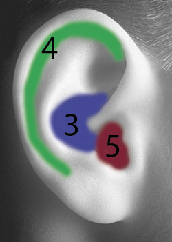 Colored lines in the graph above represent acoustic gain contributions from various parts of the ear itself. The blue line represents the focusing effect of the concha bowl into the ear canal of sound in the mid-treble region (with a peak at about 5kHz). The green line represents contributions from the pinna flange, which are somewhat lower in frequency due to being farther from the ear canal opening than the concha, and lower in level due to the milder cup shape of this area of the ear. The ear canal and ear drum resonance is represented by the red line (5), and shows its first resonant peak at about 3kHz (1/4 wavelength of ~1" long ear canal). If you were to extend this line further you would also see resonances at about 9kHz (3/4 wavelength resonance) and 15kHz (5/4 wavelength resonance).
Finally, we can sum all these gain contributions together to get a full picture of the differences between what a measurement mic hears in free space and what your ear drum hears when you place your body in front of a speaker. The solid black line labeled "Ear Resonance" shows the sum total acoustic response present at the ear drum. Another way to think about it is the acoustic transfer function of the ear, head, and torso. Because our brain is used to hearing with this response, it sounds flat to us. When we measure headphones at the ear drum, we are not looking for a flat response, rather, we are looking for a response similar to the curve in the graph above. We'll call the curve we're looking for the Headphone Target Response Curve (HTRC).
Unfortunately, there are some significant problems figuring out the exact HTRC to use.
Individual Variations
Most obvious is that fact that all these specific response curves are generated by a specific geometry in the shape and size of a person and their specific ear shape. The particular graph used above is probably an average of many people, but the fact remains that your specific body, head, and ear shape will likely produce a different response curve at the ear. The Head Acoustics head I use for headphone measurements has an ear specified by international standards (IEC 60318-7:2011) to be exactly average for all humans, but it too will differ from your ear response.
So, this is the first thing to know about headphone measurements: They were not made with ears the same size as yours, so the sound you hear may objectively be somewhat different than the measured values. There really isn't much that can be done about this. For the sake of accuracy and relative consistency some one human looking ear needs to be used for all measurements, it seems to me the use of a standardized average ear is a good option. I wouldn't say the magnitude of this problem is huge—after all we're all listening through human ears that do have significant commonalities—but I do think the differences could be enough for the same headphone to sound audibly different (mostly in the treble area above 2kHz) on two different people.
Sound Source Direction and Acoustic Environment
This is where things get very complicated (as if it hasn't been complicated enough already). In the above "Acoustic Gain Components" graph we've been using so far, you'll notice at the top left that this graph is for sound coming from a 45 degree angle. I'm pretty sure this graph was also done with a flat speaker in an anechoic chamber. If you change the angle of the speaker relative to the head, the geometry of the torso, head, and ear changes relative to the acoustic wavefront, which will in turn change the acoustic resonances and the associated peaks in response.
Also, if you take a speaker that measures flat in an anechoic chamber and put it in a normal size room with typical acoustic characteristics, it will sound (and measure) somewhat warmer as the room's volume reinforces bass notes (usually below 200Hz), and the speakers radiated power into the room decreases as they get more directional at high frequencies (results in aproximately 3dB tilt between 200Hz and 20kHz).
To summarize: the target response curve at the ear drum will change significantly as you change assumptions about the direction of the sound source and the acoustics of the room you're in.
Historical Target Response Curves
The world of audio engineering has historically had only two standardized ear drum response curves: Free-Field (FF), and Diffuse-Field (DF). The FF curve was the population averaged measured response at the ear drum for sound coming from directly in front of the listener in an anechoic chamber. The DF curve is the population averaged measured response at the ear drum for sound coming from all directions simultaneously in a very reverberant (hard-walled) environment.
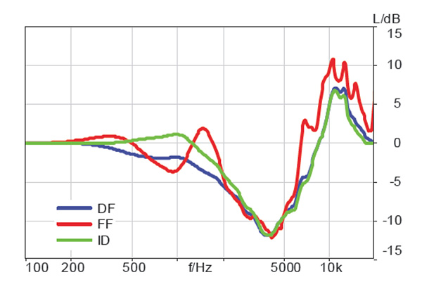
The graphs above are simplified versions of the compensation curves for the Head Acoustics HMSII measurement head I use. You can see these curves are similar, but upside down, relative to the ear drum response curve we've been looking at. That's because these are compensating curves intending to reverse out the ear drum response and bring it back to flat. (The Independant of Direction curve is one invented by the company and is not an internationally adopted standard. It is essentially a DF curve with some of the head and torso effects taken out of the calculation. It is the compensating curve I use for InnerFidelity graphs.)
Historically, the DF curve had been generally adopted as superior to the FF curve as a target response curve for headphones. But over time, and largely due to discrepancies between the objectively derived DF curve and other subjectively developed target response curves, headphone makers have been moving away from the DF curve as their target response for headphones.
What makes sense as a target response curve?
I've been trying to make good headphone measurements for about twenty years now. I've given this subject a lot of thought, and the answer has always seemed simple and obvious to me: If music is mixed and produced to be played back on speakers, and if good headphones are suppose to sound the same as good speakers with recorded music, then the target response curve should be the ear drum response of a human head and torso in front of two ideal speakers in an ideal acoustically treated room of about living room size. In simpler terms, I've always thought that good headphones should sound like good speakers. It just makes sense.
The approach then would be to put a measurement mic in front of two very good speakers in a very good room and take a baseline measurement. Then place a measurement head in the same position and take the ear drum measurement. Then subtract the baseline room measurement from the ear drum measurement and you've got a new target response. Unfortunately, that is a lot easier to say than to do. To make that measurement very well there are a number subtle nuances to the measurement (like spatially averaging the response over a range of listening angles) and very expensive equipment and well trained operators are needed. This is an expensive undertaking to do well, so there had better be a darn good reason to go to the effort. My internal hunch is probably not a good enough reason. Fortunately, I'm not the only person to have this hunch.
Harman Target Response Curve in Development
I won't go into too much detail in this article as I've written extensively about it, but researchers at Harman International lead by Dr. Sean Olive have been working diligently for the last couple of years on defining a new headphone target response curve. Their very thorough research has lead them to the basic conclusion that headphones should sound like good speakers in a good room.
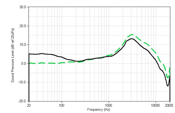
Green dashed line is the ear drum response of a speaker that measures flat in the room. Black line is the subjectively derived preferred ear drum response for headphones.
The graph above shows the ear drum response as measured on a dummy head at the normal listening position between a pair of speakers. The green dashed line shows the ear drum response for a speaker that has been equalized flat at the listening position. The black line shows the adjustment away from flat while wearing headphones that most people chose as more pleasing.
There are a couple of nuances to understand here. First, most speakers are designed to measure flat in an anechoic chamber. When a speaker is put into a room it gets a bass boost from the proximity of the walls—this boost typically happens at about 200Hz and below. It also naturally gains a warm tilt due to the ever reducing sound power being put into the room as the frequency gets higher and the speakers directivity becomes more narrow.
The important thing to take away from this is that the goal is not actually for flat sound in the room. The goal is actually for the slightly warmer sound of speakers designed to be flat in an anechoic chamber and how they interact with the room. One of the underlying suppositions here is that we humans know what a room does to sound, and we accept—in fact, expect—that the sound from a good speaker will change in the room.
Another interesting subtlety in the research was that while the ear drum target response curves for speakers and headphones were quite similar, people actually preferred slightly bass and treble on headphones than they do on speakers (about 2dB on either end).
Headphone Frequency Response Measurements
 And now, finally, we can talk about what to look for in a headphone frequency response measurement.
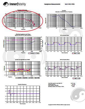
The top left graph on each of the measurement pages is the frequency response plot. You'll see two sets of response plots on this graph. The bottom set is the raw measured ear drum response of the headphone. I make this measurement five times and slightly move the headphones each time. All ten (five left and five right) are shown. The reason for doing this is that the measurement will change as various resonances change as the position of the ear within the headphone moves to different positions. By taking five measurements I can average them all together and remove some of these changing resonance artifacts. This is called spacial filtering.
The top plot is the averaged raw responses compensated by the Independent of Direction compensating curve that came with my measurement head. Over time I've come to look much more at the raw, uncompensated curves than the compensated plot, primarily because I know the ID (or DF or FF) compensation curves are not quite correct.
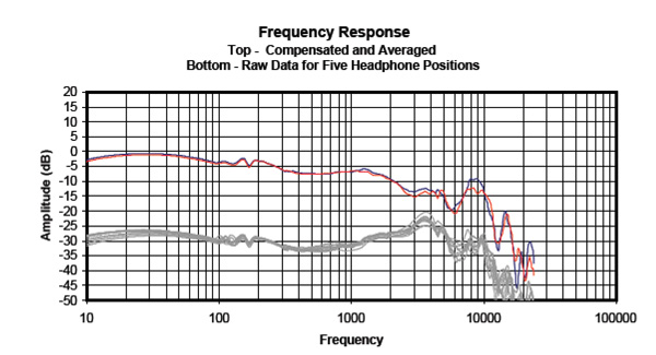
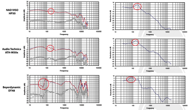
Frequency response plots for the NAD VISO HP50.
When I look at the frequency response plots above with an eye towards understanding its tonal balance, I am primarily looking at the raw response plots and mentally comparing them to what I understand of the Harman Target Response. The NAD VISO HP50 above is quite close, as is the Focal Spirit Profesional.
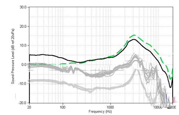
In the image above, I've crudely superimposed the raw FR plots of the NAD VISO HP50 (top gray lines) and Focal Spirit Professional (bottom gray lines) on the chart showing the preliminary Harman target response curve (black line). These two headphones are among the most neutral I've heard, and they do match the Harman target response quite well relative to other headphones I've measured.
One thing you'll notice with both these headphones is that the rise into the bass starts at about 400Hz, while the rise into the bass on the Harman response starts at about 200Hz. This causes the bass to mids transition to be a little too thick or overly warm sounding, and is quite common with many headphones.
Someday, I will convert my compensation curve to something like the Harman target response, until the you'll just have to use your imagination and keep the preliminary Harman curve in mind as you look at the raw plots. I've created this image to give you some numbers to remember as you evaluate the raw frequency response plots.
We'll get into some of the specific characteristics to look out for in headphone measurements in part 2 of this article, but it's important to note early on that high frequency measurements are dominated by the wild swings of the resonant behavior of headphones. When you look at the profile of the frequency response curve at the high frequencies, you need to mentally average out all the peaks and dips to an average level to get a good feel for what's really there.
A Side Note About Other Headphone Measurement Systems
In the current article, I've been quite insistent on the importance of industry wide headphone measurement standards and instrumentation. It is of crucial importance that standards become adopted as it allows industry participants to operate on an apples-to-apples basis, and it allows for more efficient further progress in areas of research. The problem with this gear is that it's exquisitely expensive. Last time I checked, artificial heads like mine were around $25k by the time you got all the options properly sorted; and the simpler couplers were in the $7k region. Accuracy is expensive.
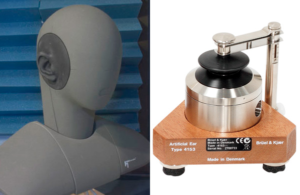
Above left is the Head Acoustics HMSII head and torso simulator used to measure headphones here at InnerFidelity. Above right is the B&K 4153 artificial ear simulator. Both instruments comply with international standards and will deliver substantially similar measurements when measuring the same headphones.
However, if you've read the above article carefully, you'll see that even with extraordinarily expensive equipment, accuracy is hard to come by. For many hobbyists who simply want to keep objective track of headphone modifications or want to do some basic headphone comparisons, home made headphone measurement systems are possible. A couple are mentioned in this article. I think this is an absolutely terrific hobbyist activity. (I didn't have a lot of time to research it, so I would love it if any InnerFidelity readers who have made their own measurement systems and written about them post links to your gear in the comments. Thanks!)
But it's important to recognize a few things about those measurements vs. the measurements from industry standard compliant instrumentation. Some hobbyist systems are designed to approach industry standard compliance, but many are not and aren't attempting to. Measurements taken on these various systems of a particular headphone model may be substantially different and should be considered apples-to-oranges comparisons. The only time you can even begin to compare headphone measurements from different systems is when industry standard compliance couplers are used. Even then, different operators will place the headphones on the couplers a little differently yielding varying results. Some manufacturers prefer to make measurements that will be presented to the public on the Neumann K100, a head shaped microphone that makes roughly flat response measurements for roughly flat headphones, but not compliant with headphone measurement standards.
The point is, all the advice in this article is only true when you're looking at headphone measurements taken with standards compliant instrumentation. And, if you're going to compare headphone measurements, always compare measurements that have been made on the same system. It's also helpful if you are going to look at any set of measurements to get used to the way that particular lab's measurements appear. To really get the feel for this stuff you have to spend a lot of time listening to headphones while you're looking at graphs. There's some good learning available there...but beware, there's also ample opportunity to create your own little rabbit hole of expectation bias.
On the other hand, measurements are the one thing you can look at with a sense that some truth is there to be had. Measurements are real...how meaningful they are isn't easy to answer, but we'll keep plugging away at it.
Target Response
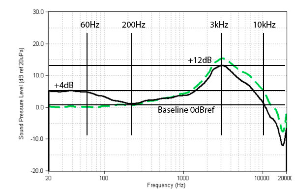
Earlier, I introduced a bunch of concepts that resulted in a target headphone response curve (as measured at the ear drum) that looks something like the black plot above. (The green plot is what speakers, equalized to be flat in the room, look like at the ear drum.) To some extent, it's necessary to memorize certain aspects of the curve above in order to be able to mentally compare it to the raw frequency response plots when you look at headphone measurements. The first thing to do is establish a 0dB reference level, which should be the lowest point, or the average level, of the mid-range (~200hz-1kHz) on the raw frequency response plots. These are the characteristics you should look for:
- +4dB rise in the bass, starting no higher than 200Hz and at full level by 60Hz.
- From 200Hz to just over 1kHz, you should have a gentle 3dB rise.
- The main peak of the plot should be at 3kHz +/-500Hz ideally. If the peak starts getting too high in frequency the sound can get quite piercing in nature.
- Although the curve can get fairly noisy above 3kHz, it should generally follow the profile shown and be roughly back to 0dB at 10kHz. And a less noisy frequency response curve is generally better sounding.
- Above 20kHz the plot should continue to fall off to about -13dB below baseline.
The above curve is right out of Sean Olive's paper "Listener Preferences for In-Room Loudspeaker and Headphone Target Responses" and my notes above are for that curve. My personal sense is that it's close but not quite right. So here are a few variables to consider:
- I think the bass may be high by a small amount, I'd rather see 3dB in the bass. I do agree that the bass emphasis should all be below 200Hz, any higher at all, and you start to hear the lower mid-range start to thicken up unnaturally.
- The 3dB rise from 200Hz to 1.2kHz is so rare that I really can't say much about whether it's right or not. This rise mainly comes from the head and torso interaction that is bypassed by headphones, so I would think it's something that should be there on headphones, but it might be very difficult to achieve.
- I think +12@3kHz might be a a few dB high. I'd say you want this peak between 10dB-12dB, but not higher lest there be daggers in your ears.
- Although headphone measurements may be noisy and have lots of peaks and valleys above 3kHz, on average it is good to see the level back to between 0dB and 3dB at 10kHz. It is very common to have a peak in response near 10kHz due to an ear canal resonance; this peak being higher than the average level can be okay if nearby frequencies remain near the target curve level on average.
- It is very difficult to get a real sense of where the levels are above 10kHz since measurements are so noisy and plagued with resonance artifacts, but my sense is the Harman response curve shows too much roll-off. I think that while levels above 10kHz should continue to fall, the drop should be more like -10dB.
Okay, lets take a look at headphones that approach the above curve, and some that don't, and what that means when relating measurements to the listening experience.
Later, will also look at some of the characteristics of ear pads that can be seen in the frequency response curves; characteristics that are unique to in-ear monitors; and a few other odds 'n ends that can be seen in the frequency response plots of headphone measurements.
Historical Headphones Relative to the Target Response Curve
The point of this section is not only going to be identifying headphones that approach the target response, but also noting how they deviate from the curve and what character it might give the headphones apart from sounding neutral. Remember, we're going to be talking primarily about the lower gray curves that are the raw frequency response measurements from the dummy head with microphones at the ear drum position. (The upper blue and red curves are compensated.)
Lets start with a few headphones that have historically been considered "good" sounding.
Sennheiser HD 580
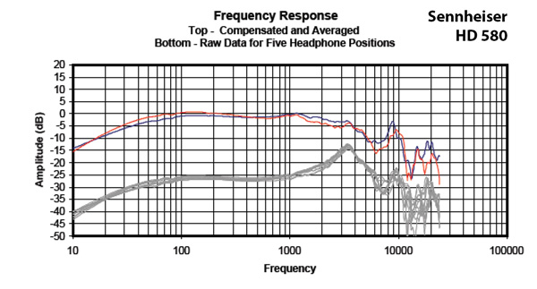 For this plot, we'll call the -25dB line the 0dB reference. You can see that the peak at 3.3kHz and +12dB over baseline is just about right when compared to the target response curve at the top of the page. The fall above 3kHz is somewhat too steep with the peak at 10kHz just reaching the 0dB line, and the average falling significantly below. This would cause the HD 580 to sound somewhat laid back, and, of course, this headphone is famous for having very good, but "veiled" sound.
You'll also note the bass is not accentuated but is, in fact, rolled-off in the low bass. Fifteen years ago headphone enthusiasts really didn't complain of the HD 580 not having enough bass; that kind of response in headphones was the norm. We were used to it.
AKG K701
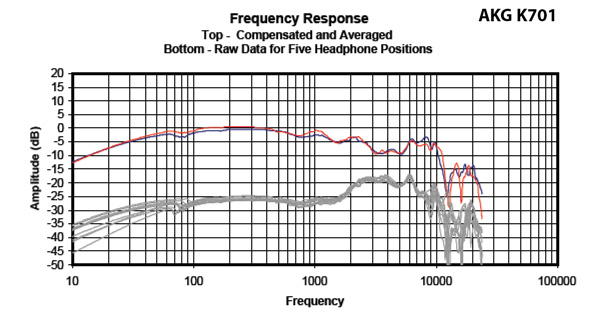 Another old favorite is the AKG K701, which generally considered a brighter headphone than the HD 580 but still fairly neutral when it was first introduced. Here you can see there is no well defined peak at 3kHz and that area only rises about 8dB above baseline. More importantly, above 3kHz it continues at +8dB to 5kHz before beginning to descend to baseline around 10kHz. There's quite a bit more treble energy in the K701 than the HD580 above 3kHz relative to each other.
You'll also notice the broad mid-range hump is centered at about 300Hz, while it's centered at 120Hz on the HD 580—that's more than an octave higher in music, it's quite a bit of difference in the overall center of emphasis. This makes the the bass sound just a bit warmer on the 580 than the overall cooler sounding K701. The point here is that the K701 and HD 580 clearly sound different while there measurements are not that dramatically different. Subtle interpretation is important to get things correct.
Beyerdynamic DT 880
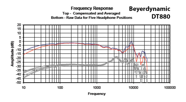 We might as well have a look at the Beyerdynamic DT 880 as it joins with the first two as the triumvirate kings of the headphone hill for quite a while. Here you can see that the DT 880 has quite similar response to the HD 580 to 3.5kHz. Above 3.5kHz the DT 800 remains high and the 10kHz peak is at +10dB relative to baseline, with an average level at about +3dB at 10kHz. Energy above 10kHz is about 5dB higher than either the HD 580 or K710. The DT 880 was a bit brighter sounding than the K701.
Denon AH-D5000
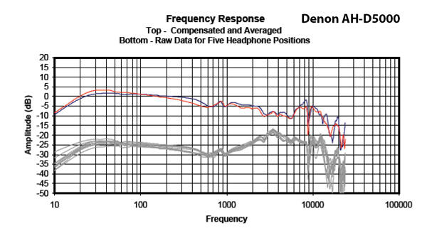 Another old school headphone that had a strong following for its good sound is the Denon AH-D5000...and its siblings D2000 and D7000, which were similar. While it doesn't have the step up in the bass of the target response curve it at least does rise about 5dB from baseline, which gave this headphone a sense of heft and body the the first three lacked, and which was broadly appreciated by enthusiasts.
Unfortunately, while the 3.5kHz peak is in a good place 12dB above baseline, it subsequently looses little energy and remains 5dB above baseline to about 13kHz before dropping. This made these headphones somewhat too hot in the treble for some listeners (me included), and was particularly noticeable on the D2000.
Sennheiser HD 800
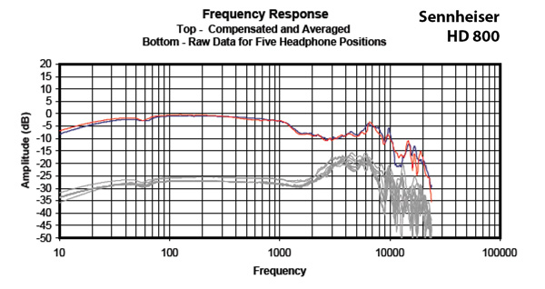 Introduced in 2009, and remaining still one of the finest reference headphones on the planet, the Sennheiser HD 800 shows some improvements over the HD580/DT880/K701, but also some troubling features. The bass response doesn't roll off as fast as the first three, which gives the HD 800 a stronger punch down low. The rise to 3kHz is good and the subsequent response has fairly good shape without excessive peaks and valleys. However, everything above 3kHz is also about 3dB too high as well, making these a headphone that can be too bright for comfortable listening.
Audeze LCD3
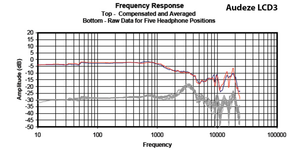 Then about five years ago we started hearing planar-magnetic cans and people were immediately drawn to their powerful and tight bass response. The graph above shows the LCD-3 with a wonderfully flat bass extension. Even though it's below the target response, it's much flater and better extended in to the lowest notes than anything that preceded it. People love planar magnetic headphones for their well extended bass response. I have to say though, after having spent some time now with headphones that more closely conform to the base boost of the target response, I do feel that it's more pleasing, and a more subjectively accurate representation of neutral.
The plot above is from one of the earlier LCD-3s that were considered somewhat lush in the mids and polite in the treble. In the plot above we do see a slight rise from 200Hz to 800Hz, which gives the sense of strength and character to the vocal harmonics. But the subsequent dip before the peak at 3.5kHz puts the LCD-3 a little off the pace in the presence region—the sound of spit on the lips or saliva on the reed of a sax is going to sound a little laid back. Also, above 3kHz it falls too quickly and, other then the level of the 10kHz peak, is about 5dB below the target curve. All this might make for a headphone that is too polite in sum, but the treble above 10KHz actually rises above the target and somewhat makes up for the slightly too dark treble otherwise.
Two things to note here. First, this is where the value of measurements end, and only experience can fill in the blanks. Yes, the LCD-3 is a bit too low in the low and mid treble (though the peak at 3kHz is the right height), and a bit too hot in the top octave above 10kHz, but it's not too far off. The question is: does that sound bad or good? Because it can go either way. And second, we're only looking at the FR measurements and not able to analyze all the other plots. There are further hints about sound quality gained by looking at transient and distortion characteristics, but there again there are limits to how much information about the quality of the listening experience that can be gleaned through measurements.
Stax SR-007
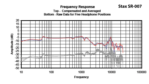 Last old school headphone that needs to be viewed would be a Stax electrostatic. Many would say the SR-007 shown above is the best of the lot.
I'm not certain, but I would assume the drop in the bass is due to a pad resonance. Electrostatics have a reputation of having poor punch in the bass, but I think that's a bit of an overstatement. I think there has been some problems with pads and how they fit historically, and I do think that larger electrostatic panel speakers may have had poor bass impact, but from what I've heard and can tell from measurements, electrostatic headphone have fairly good bass response; certainly as good or better on average than open dynamic headphones.
Above 200Hz the curve does have a nice rise to 1kHz, but subsequent rise to 3.5kHz is a bit of a roller coaster and on the low side of optimal at 8dB over baseline. The fall after 3.5kHz starts off about right but at about 8kHz begins to gather about 5dB of energy and keeps that emphasis for the remaining treble. Like the LCD-3, Laid back in the lower treble ranges, hot in the top treble ranges, but overall close. It's just how it all comes together in you ears that will determine wither it's good or bad for you.
Current Headphones Close to the Target Curve
The next group of plots will be from current headphones that I've measured and appear to come close to the target response curve. They all sound fairly good, in my opinion. That's not to say there arent good sounding headphones that farther off the target curve, or headphones that may be close to the curve but sound poor, I'm just saying the headphones on the target curve seem to have a pretty good probability of sounding good.
NAD VISO HP50
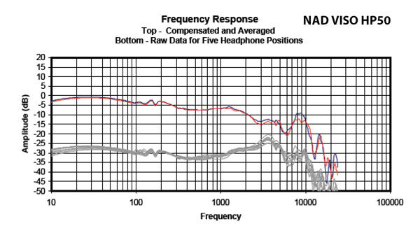 The first headphone that I've measured that had a raw response very close to that of the target response curve is the NAD VISO HP50. Paul Barton designed this headphone with a very clear picture of the acoustics and studies surrounding the development of target response curves in general. He went straight to the drawing board with his own target response curve using the trademarked term "RoomFeel." The result is a headphone with a very pleasing and fairly neutral sound, and a measured performance quite close to the Harman target response.
In the plot above, you can see that though the bass has a very typical broad hump characteristic of dynamic headphones, there is an overall rise of about 5dB over baseline. The transition upward into the bass starts at about 400Hz, which is a bit high in frequency and will typically cause a bit of thickness to appear in the low mids. From 500Hz up to 3.5kHz we see a beautiful profile that very closely fits the target response and indeed the HP50 does a very nice job of rendering vocals with a natural timbre. Though there's a dip at 6-7kHz and a small peak at 10kHz, the overall profil of the upper treble on the plot matches the target response well.
It's probably a good time to note that a dip somewhere between 5-8kHz in response might actually be preferred to the Harman target response in the region. Work by Philips on the X2 headphone suggested to them that a notch in this region is subjectively preferred. Too much energy in this area can be quite abrasive to the ears. I don't know this for sure, but if you see a dip in the 5-8kHz region it might be a good thing.
Another thing to start noticing as we look at cans that have good matching with the Harman curve is the shape of the compensated curve. As I mentioned in part one of this article, I use the "Independent of Direction" compensation provided by Head Acoustics, which is quite similar to the "Diffuse Field" response. One thing you'll notice is that if a headphone closely matches the Harman curve, it results in a relatively featureless sloping line that gradually drops of faster as you go higher in frequency. The one exception is the peak at 10kHz, which can be overemphasized by the compensated curve.
Focal Spirit Professional
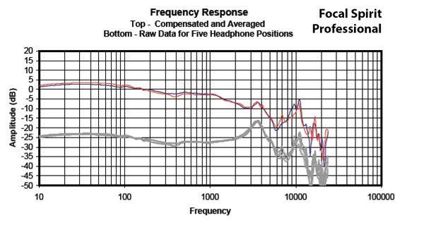 While the Focal Spirit Pro plot below 3kHz is a little smoother than the HP50, it doesn't do quite as good a job of producing the long linear rise from the mids to the 3kHz peak. It's more liquid and coherent sounding bass through mids, but it's also a tad polite in the presence region sounding a bit more laid back than the more correct to my ears HP50.
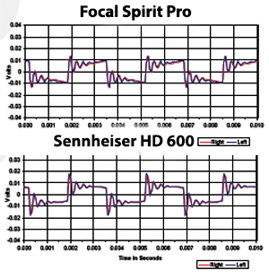 The valley at 6-8kHz, peak at 10kHz, and subsequent peaks and valleys are not optimal, but after having looked at hundreds of headphone frequency response plots I've found that this feature is surprisingly common and often fairly benign. I'm going to break my rule about remaining with frequency response plots only, and show the 300Hz square wave for the FSP and HD600 (which has a similar look to its FR plot). You can see that rather than a clean initial step there is some ringing. I don't know for certain, but I think this may be a fairly natural result of ear canal resonances due to the way some headphones acoustically interact with the ear, and it might be that the auditory perception system knows how to ignore it. In any case, when you see the a frequency response plot with three big peaks at 3kHz, 10kHz, and 15kHz, and the triple ringing front end of the 300Hz square wave, it's a good bet that while the treble may not have superb transient response it will probably sound okay. This measured feature seems to look worse than it sounds.
Shure SRH1540
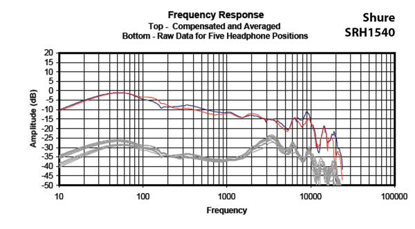 At first glance the Shure SRH1540 looks quite a bit like the target response curve. The bass boost is nicely placed with a start to the boost at 180Hz, but at +8db over baseline at 50Hz is a tad excessive. The peak at 3.5kHz is of proper height, but lacks the long slope upwards from 200Hz, causing it to loose some presence and richness of vocal overtones. The decent of the treble above 3kHz has fairly good shape, but should probably fall of a little faster and be down another 3-5dB at 20kHz.
In short, it's got a bit too much bass and high treble, and lacks a bit in the mids—a mild "U" shaped response, and that's exactly the way it sounds. One thing worth mentioning here is that while a "U" shaped response may be too exciting for some (me included) at solid listening levels, it tends to sound great at lower volumes as it delivers a bit more bass and treble, just like Fletcher and Munson prescribe. So, if you listen a lot at low levels (as I often do) this is a terrific headphone.
All the headphones above are around-the-ear, sealed headphones, which seem to be the most likely type of can to get close to the target response—especially in the bass—but there are a few headphones of other types that get close.
Philips X2, circumaural, open
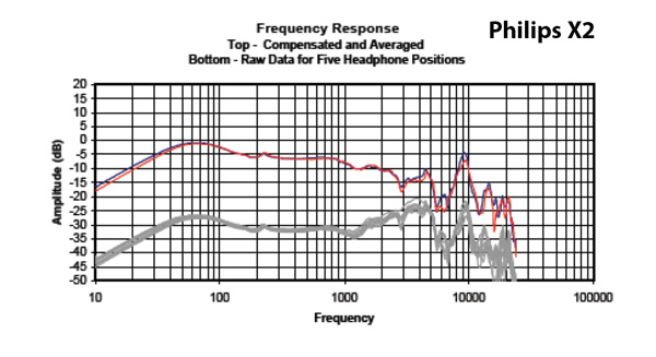 Open, dynamic driver headphones have a much tougher time getting the bass extension of sealed dynamic headphone, and you can see that the X2 does fall off at about 6dB/octave below primary driver resonance at about 60Hz. However, unlike the three open headphones at the top of this article, the mid-range is not a broad hump but rather is flat with a hump only below 200Hz. This is a fairly good approximation of the target response for an open headphone.
The mid-treble peak has about the right level, but centered at 4.5kHz is a bit high. However, this headphone was designed with a lot of feedback from trained listeners, and it was determined that a notch at 6-8kHz makes for better listening. This notch could very well have required a bit more energy both before and after to help compensate for the loss of treble energy in the notch. The result is a nice, warm, friendly sounding headphone, but I think all the tuning to get the curve into the desired shape has caused the response to lack a little smoothness and, as a result, sounds a bit grainy to me.
V-Moda XS, on-ear, sealed
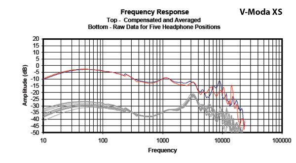 The XS has a somewhat excessive bass response that bleeds too far up into the mids giving them a bit of thickness to the sound. But the fact that the rise to 3kHz starts below 1kHz, and the fall above 3kHz (though starting off a bit fast) has good proportion makes for a really lovely sounding headphone.
V-Sonic GR07 Bass Edition, dynamic driver, in-ear
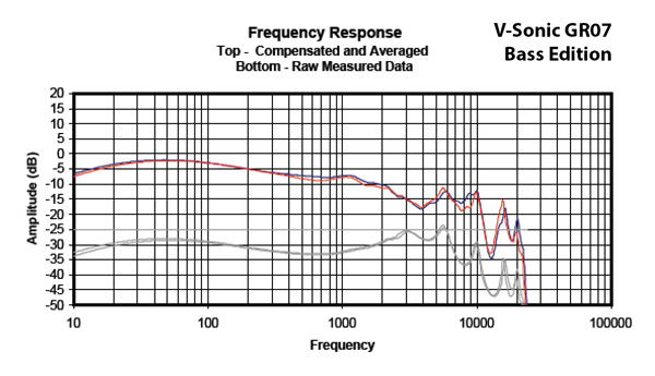 This is a headphone I heard only briefly after measuring it and seeing such good measurements, so I really can't comment in depth. ljokerl can however, and in his GR07 review on TheHeadphoneList.com he gave the GR07BE a 9.1/10 in sound quality.
One thing I will point out however is the peak at 5kHz being equal in level to the one at 3kHz, which might skew these headphones into sounding a tad bright. ljokerl's comment at the end of the review has him pointing to "Mildly sibilant on some tracks" as one of the GR07BE's cons.
Here are a few more IEMs that measure relatively close to the target response. I'll just post them without comment.
Headphones a Little Farther Off the Mark
The above headphones are about all there are that are very close to the target response curve. Let's look at some fairly good sounding headphones that are a little farther off the curve and see if their failings match their deviations from the target.
Beats Solo2
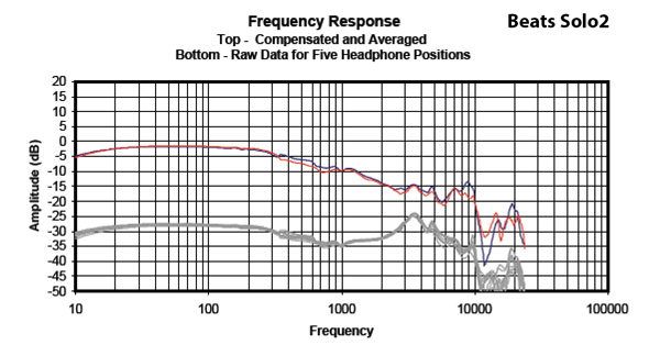 A big round of applause for Beats getting this damn close to the target response, the new Beats Solo2 is a good sounding headphone—WAY better than the first Solo. However, you can see that the bass boost goes all the way up to 500Hz, which causes the low mids to sound quite thick. And while the peak at 3.5kHz and subsequent drop to 10kHz look fairly good, the drop between 10kHz and 20kHz is far too excessive, causing the headphones to lack a sense of spaciousness.
AKG K267 Tiesto
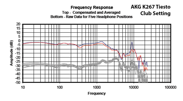 The K267 has a switch on the earpieces that changes the internal acoustical tuning to adjust the bass to three different settings. In the "Club" setting it does a fairly good, if a bit rough, job of mimicking the target response, especially in the long rise to the 3.5kHz peak from ~300Hz. It has a fairly wide notch above 3.5kHz, which may sound okay, but it does seem a bit too wide to me. Above about 8kHz the curve looks good.
Musical Fidelity MF100
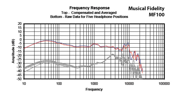 When I first saw my measurement system draw out the plots for the Musical Fidelity MF100 I was giddy with excitement, it looked like it was very close to the target response. But as you look at it a little more closely, you'll see the 3.5kHz peak is about +3dB too high, and the subsequent run up too 10kHz remains far too high in level. In listening this headphone sounded mostly good but somewhat piercing to me, and caused me to put more credence on Philip's idea that taming the 6-8kHz area might indeed be a good idea. The MF100 is a bit hot there and suffers dearly for it. You may also want to take a peak at the full measurements to see how this treble boost made for a very significant leading edge spike. So, close, but no cigar.
Audio Technica ATH-M50x
 Though pretty rough looking due to some pad bounce artifacts between 80Hz-300Hz, the M50x response is quite close to the target curve from 20hZ to 4kHz, especially between 300Hz and 3kHz, and this is indeed a good sounding headphone. Above 4kHz is a notch probably too large, but response is in place above 10kHz. Overall, the tonality of these headphones is excellent, but, as evidenced by the herky-jerky response, they aren't particularly refined or liquid sounding.
Okay, that's probably enough on the target response curve, let's turn the page and look at some of the other things that can be seen in the raw frequency response measurements.
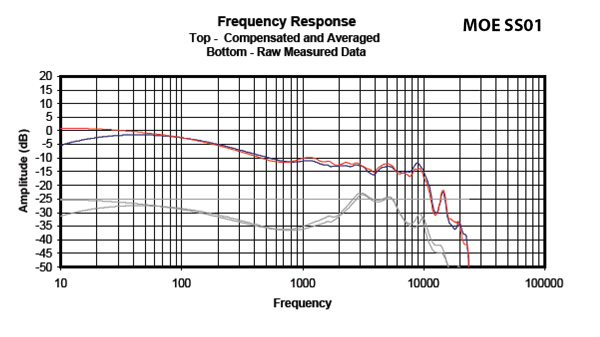
In-Ear Monitor Response
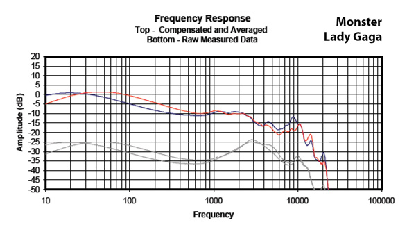
As you saw in the target response area above, there are some IEMs that get close to the target response, and they are considered good sounding. There are a number of valid reasons to believe that the target response measured at the ear drum for IEMs may be somewhat different than regular headphones, but, I know of no reason to think it's way different. Just like research shows that the target response measured at the ear drum for headphones and speakers is different but only by a few dB, I'm pretty sure we'll find that neutral on headphones will look very much like neutral on in-ear monitors. In other words, IEMs that sound good are not going to measure +15dB louder in the bass than the target response with a bass boost that extends to 800Hz. And that, unfortunately, happens all too often.
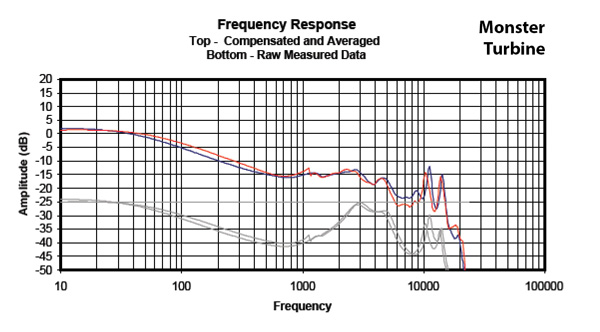
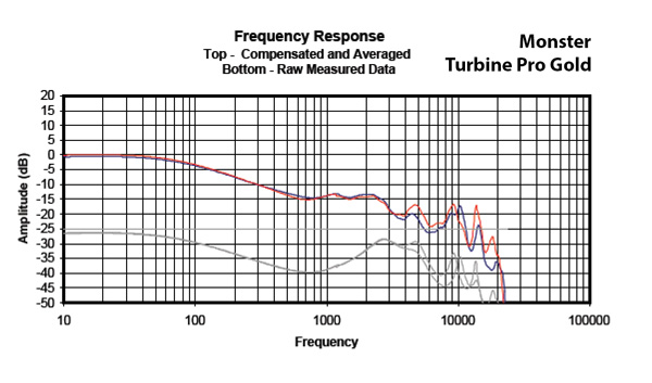
Another thing you can see in the above plots and on many IEMs is the level of the peak at 3kHz is about +15dB over baseline, when it should be more like between 10dB-12dB. It's interesting to note that the 3kHz peak in the Monster Turbine in the graph just above this paragraph, is about 3dB higher than the corresponding peak in the Turbine Gold shown below—the Gold intended to be a more premium headphone, and which did sound better to my ears in the treble, though the bass was still too much.
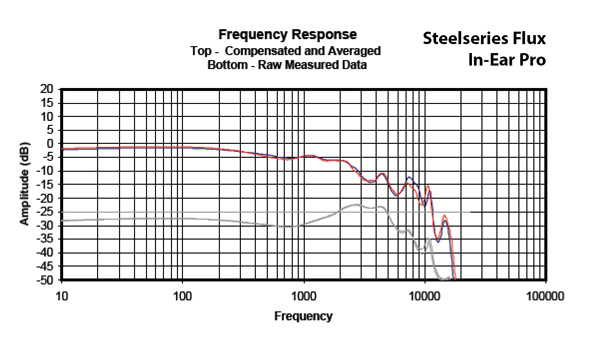
Another common characteristic of IEMs is a series of sharp peaks in the treble. These are caused by the resonance of the trapped volume in the ear canal and tubing within the ear-piece. In my experience, they tend to be somewhat benign if not excessive, and if on average they follow the contours of the target response.
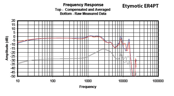
The Etymotic ER4P in the plot above is famous for having a very clean and well balanced treble. You can see that even it has some significant peaks in the high treble.
Pad Bounce
I'm sorry, I haven't come across some official term for this, so I'll just call it pad bounce for now. It boils down to the springiness of the pad and enclosed air volume against your head creating a low frequency resonance excited both by the acoustic energy in the ear cup and the moving mass of the driver. It shows up as a little wiggle in the frequency response, usually somewhere between 60Hz and 200Hz. And, interestingly, it will also show up on the isolation plot (measuring how much the headphones attenuate outside noise) as an amplification of outside sound as the headphone begins to bounce along with an outside sound at the resonant frequency.
The above plots show three cases of pad bounce from mild to severe. To my ears this artifact is not terribly disturbing if modest in level, but it will contribute to a degradation to a sense of coherent, even, liquid, bass to low-mids transition.
Pad Sealing Effects
When taking the raw frequency response measurements, I reposition the headphones five times (slightly forward, back, up, down, and then centered) on the ear. I do this for two reasons: First, because it allows the various high-frequency resonances to move around a little bit, and become averaged out when the compensated curve is calculated, which produces a less confusing plot. This is called spatial averaging. The other reason to move the headphones around on the head is to get a sense of how well the headphones seal.
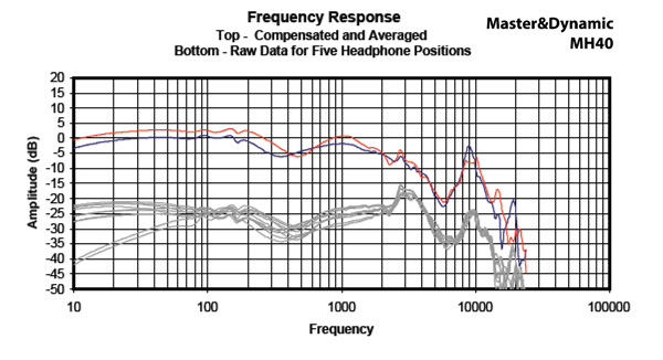 The Master & Dynamic MH40 is a headphone that requires a very good acoustic seal to get its full bass response, and it can have a hard time achieving that seal. I can remember struggling to get this headphone to seal well in each of the positions and in one of the positions it became so difficult I just gave up and let the measurement with a poor seal stand. This is where headphone measurements become less science and more art. I don't want to be unfair to the the people who use these plots and make a headphone measure better than it actually performs. When I was listening to the MH40 I did notice quite easily that it was very sensitive to pad seal and that seal would break quite easily when wearing these headphones. So, it was a conscious decision to leave the one measurement of the MH40 poorly sealed. I mention this so that if you see a measurement like the one above, with a random flier of a plot, it might not be so random.
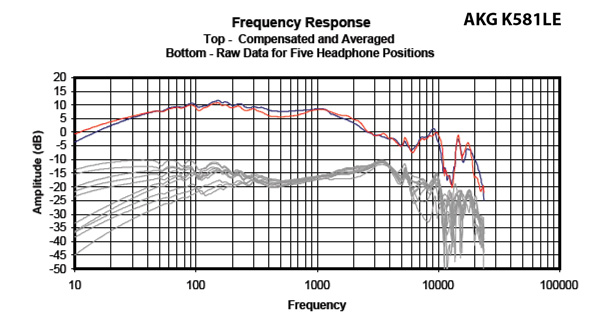 On the other hand, you sometimes get sealed on-ear headphones that are very difficult to get a good seal with and there's very little you can do to get a consistant measurement. In the plot of the AKG K581LE above (similar to a K81DJ), you can see that the seal was very inconsistant. The interesting thing here is that there's a wide variety of responses possible.
You can see that when the plots are averaged together in the compensated curve, the left and right channels balance. There's some dumb luck in this, but as I position the headphones I'm watching the 30Hz square wave response on an oscilloscope and can usually do a good job of getting the left and right channel to match—if the drivers match, and it's pretty easy to tell if they don't—which will result in the two curves matching after averaging.
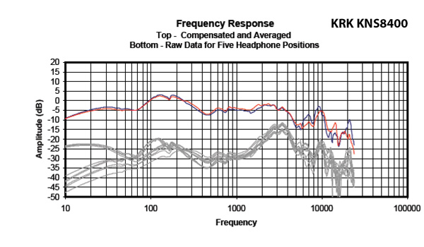 Unlike the AKG K581LE above that seems to exhibit various levels of a partial seal, some headphone either seal or don't, and the difference is dramatic. In the plot above of the over-ear, sealed, KRK KNS 8400 you can see that when it does seal the bass extends quite deep, but when it doesn't it has a significant drop off in bass response. With these headphones that require a tight seal, it's one or the other and no middle ground.
Comb Filter Artifacts
A comb filter occurs when you take a signal, delay it, and then add it back to itself.
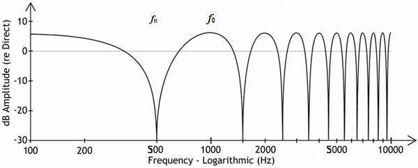 If, for example, we put in a 500Hz tone into the filter, and delay it 1mSec (1/2 wavelength at 500Hz), when we add the delayed signal back on itself it will cancel out because it's been delayed 180 degrees and is now completely out of phase with itself. Similarly, a 1500Hz signal with a 1mSec delay will put in a 1 1/2 wavelength delay and will cancel. This series of cancelations will go on every 1000Hz for a 1mSec delay, and produce a response plot looking like a series of teeth on a comb—hence the name "Comb filter".
In headphones it is possible for sound coming out of the back of the driver to go around to the front of the driver, usually through the vents in the baffle plate. When this occurs it can have a comb filter effect on the frequency response, and in my experience this can be very damaging to the sound. The comb filter effect can be seen as a series of humps in the frequency response with deep, usually narrow, notches between.
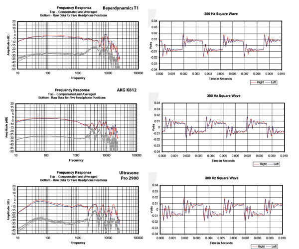
Generally, when I see this series of humps and narrow dips, it's accompanied by a really ragged and noisy transient response as can be seen in the 300Hz square wave responses in the headphones. I hear this characteristic as a glaring sound in the treble.
I should mention that there are some headphones that have single, narrow, deep notches in their treble response (i.e. Momentum). I assume these are notch filters built into the headphone by the designer to tame a certain frequency or range, and is not the comb filter response I'm talking about here.
Ear-Buds Suck
There is not an ear-bud that I've ever measured that I would consider a really good headphone. Because they don't seal in your ear canal and simply rest in the concha bowl of your ear, the acoustic coupling to your ears is very poor and variable.
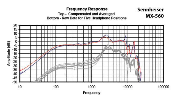 I would characterize the Sennheiser MX 560 above as an above average, but characteristically typical, ear bud. You can see that the treble response above 3kHz is actually pretty good, but everything below 3kHz is far to low in level. The treble on this headphone is about 10dB too loud relative to the mid-range, and the bass is literally off-the-chart too low.
If you have kids, you should never let them use ear-buds. The kids love the bass and they're going to try to turn up ear-buds far to loud to try to get it. The elevated treble levels in their ears can be very damaging. If you have kids I suggest on-ear, open headphones that will deliver better bass response and that will allow you to hear how loud they're playing their music. (Grado SR60, Koss Porta Pro, Sennheiser PX100.)
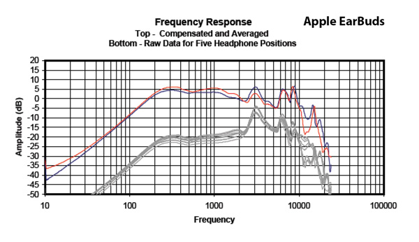
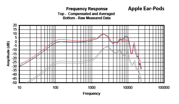
However, if you must have ear-buds, there are some good ones. Believe it or not the Apple products are quite good in this category.
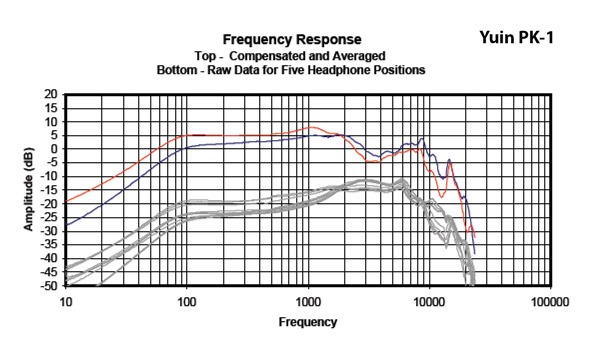
The Yuin PK-1 above is probably my favorite ear-bud...but much better sound can be had with other headphone types.
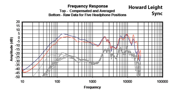
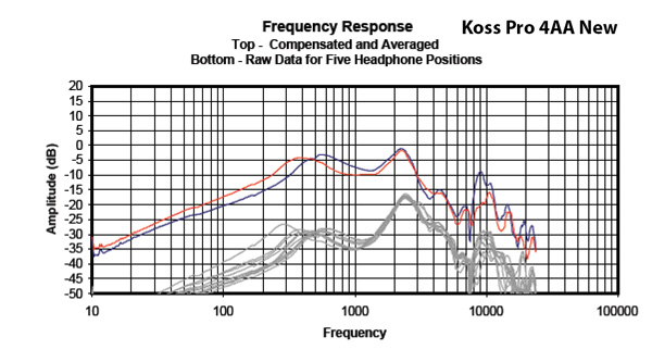
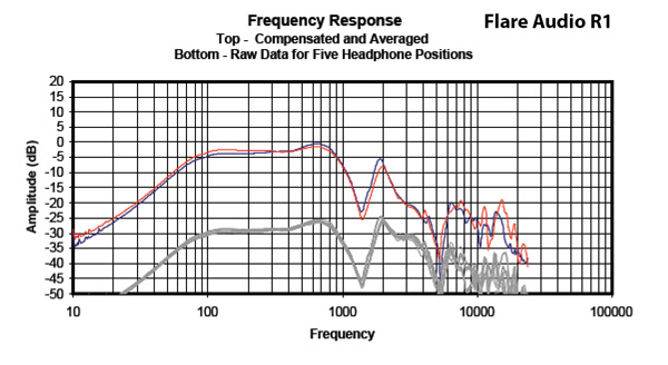
A Few Really Bad Measurements
I'm not really into public floggings, but just for a little perspective I think it's worthwhile to finish up this article with some really bad headphone measurements. By now you're probably well armed to identify the problems with these plots, so I'll just leave them here without comment. They illicit in me a sense of wonder...as in, "I wonder how anyone ever thought this was ready to leave the factory."
Total Harmonic Distortion Plus Noise
The primary goal of any audio transducer is to reproduce the signal it's receiving faithfully: high fidelity. Of course, no transducer is perfect and all alter the sound to some extent. Those alterations are distortions of the original signal. In other words, if you put in a pure 1kHz tone, harmonic distortions may cause some of that energy to apear at 2kHz, 3kHz, 4kHz etc; and non-linear behaviors (diaphragm brake-up; hair touching the driver; driver housing rattle) may cause broader band, noisy signals to apear almost anywhere in the audible spectrum.
There are numerous types of distortions and various measurement approaches that allow you to tease out the types of distortions present. The Total Harmonic Distortion plus Noise measurement method used at InnerFidelity is poor at differentiating what types of distortions are present, but very good at portraying the amount of distortion of all types present.
How THD+noise is Measured
The principle method of taking a THD+noise measurement is quite simple really. You drive the device under test (DUT; a headphone in this case) with a pure tone (called a probe tone), say 1kHz. Then, in the case of headphones, you take the return signal from the measurement head and run it through a narrow notch filter tuned to 1kHz to remove the the probe tone, leaving you with any energy in the system apart from the probe tone. This process is repeated over and over throughout the audio spectrum up to 7kHz drawing a plot of how much the headphones distort the original signal over the audio spectrum.
(The reason the plot stops at 7kHz is because at that frequency the third harmonic is 21kHz and will go out of the measurement range of the instrument by 22kHz. Once the third harmonic leaves the measurement window the measured distortion will abruptly lower even though distortion in the system hasn't actually changed. Therefor measurements of THD+noise are not internally consistant beyond 7kHz.)
Let's take a close look at the causes of both harmonic distortions and noisy distortions.
Harmonic Distortion and the Transfer Curve
Audio amplifiers have a gain curve and headphones have a transfer function, but they really all mean about the same thing. (In fact after scouring the web for a half hour I'm not sure there's an agreed upon term here...please feel free to comment about what you think is the right term.) It's a way to depict how "linear" a device is. Let's talk our way through a few transfer curves.
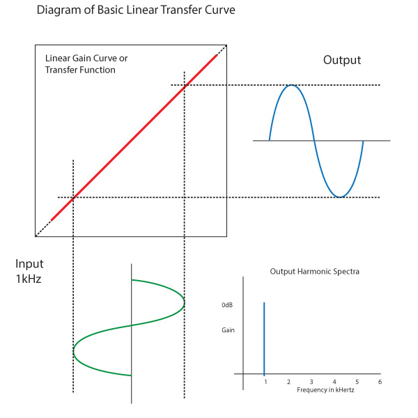
Diagram of a basic linear transfer curve.
In the illustration above, the incoming signal is in green at the bottom of the diagram. The square above it is the device under test, and the red line is its transfer curve. (For the moment let's just assume we're talking about an audio amplifier as it's a bit easier to understand this stuff for amps than it is for headphones.) As the input signal from the bottom moves left to right in sinusoidal manner, its position is projected up to the transfer curve. When viewed from the output side, this sinusoid can be seen moving up and down. Because the transfer curve is a straight line, the output signal is undistorted.
You'll also note the small frequency response plot in the lower right of the illustration. This shows the output spectra. In the case of a perfectly linear device at 0dB gain (output amplitude the same as the input amplitude) with a 1kHz input, we will see a single output tone at 0dB at 1kHz. Keep an eye on this plot as it will begin to show the harmonic distortion products as we move into non-linear transfer curves.
As I mentioned, in an audio amplifier this is sometimes called a gain curve. Not surprisingly, when we change the gain of an amplifier by adjusting the volume, we change the slope of the transfer curve.
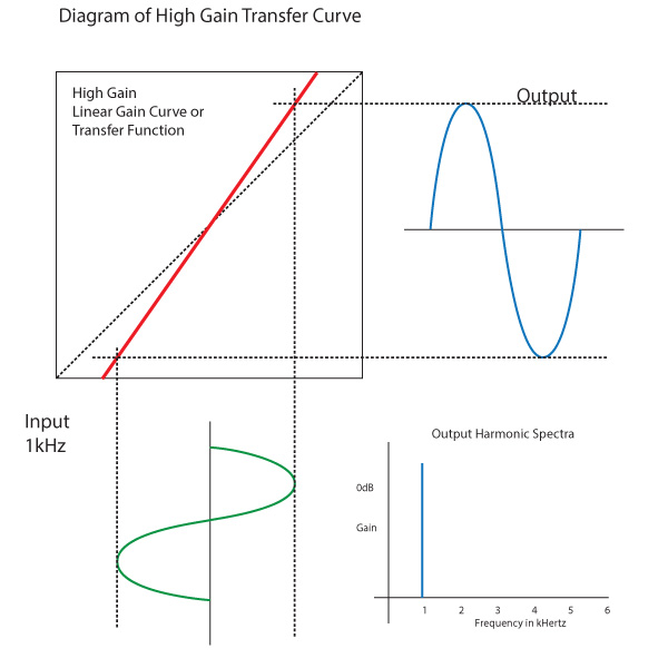
Turning the volume up increases the slope of the gain curve.
When we turn the volume of an amplifier up, we increase the slope of the gain curve. You can see in the illustration above that by increasing the slope of the gain curve we increase the amplitude of the output signal while the input signal remains the same size. The output harmonic spectra plot still shows only a single peak (because the transfer curve remains linear) but it is now at about a +3dB level.
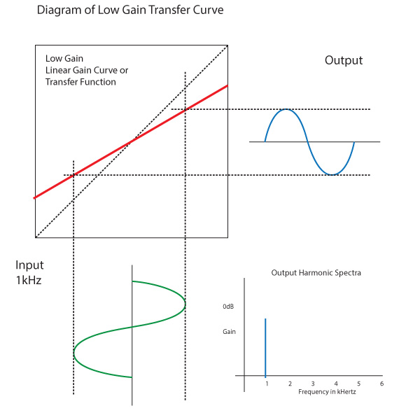
Turning the volume down decreases the slope of the gain curve.
Likewise, turning down the volume decreases the slope of the transfer curve, lowering the output level. And again, because the curve remains linear, the output shown in the harmonic spectra is a single tone but now about -3dB in level relative to the input.
Now let's imagine we have a solid-state amplifier that has +/-5 Volt power supply rails, an input a signal that's 10 Volts peak-to-peak, and we turn the volume up just a little above unity gain. Well, if the amp only has 10 volts to work with between the +5Volt and -5Volt supplies it's simply unable to produce a signal that's bigger than 10Volts peak-to-peak.
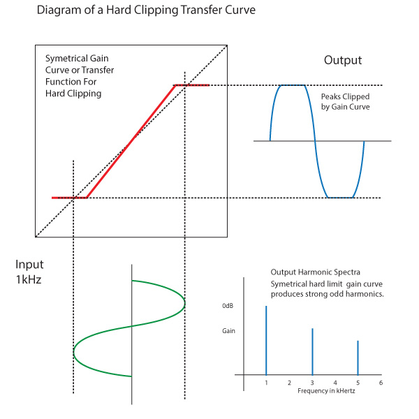
Transfer curve with flattened bottom and top similar to what might be found at the power supply limits of a solid-state amplifier.
In the diagram above you can see that the portion of the output signal reproduced on the central linear portion of the transfer curve keeps it's shape, but once the input signal reaches the upper and lower limits of the transfer curve it simply clips off the bottom and top of the waveform.
Now it's a bit complicated, but when you begin to flatten the top and bottom of a sine wave you begin to get odd harmonics. A square wave is essentially a fundamental tone and its odd harmonics at the appropriate phase and amplitude relationship. So you can see in the harmonic spectra plot that you have the fundamental tone at 1kHz, but you also have harmonic tones at 3kHz and 5kHz—the odd harmonics.
The thing to take away from this plot is that as soon as the transfer curve is anything but a straight line, you will begin to produce harmonic distortion and a series of overtones stimulated by the probe tone.
It's also worth noting at this point that if you've been around long enough to remember the introduction of solid-state audio electronics they used to make a big deal of the term "Linear Amplifier". The term linear in that phrase refers to the gain curve of solid-state amplifiers which can be made much more like a straight line than the tube amplifiers common at the time.
Speaking of tube amplifiers, they too can exhibit signal clipping, but unlike the solid-state amplifier's hard clipping and abrupt end to the transfer curve, tube amplifiers loose gain at the extremes much more gradually.

Soft clipping of an "S"-shaped transfer curve similar to that found in tube amplifiers.
The plot above shows the situation where the device under test loosing gain (reducing slope) as it reaches the extremes of its response. This would be typical of some tube amplifiers, and tends to be less abrasive sounding than the hard clipping of transistor circuits.
But what about headphones? Do they exhibit these types of response? Yes! For example, at very low frequencies as the headphone attempts to reproduce large, low frequency excursions, they begin to run out of steam on both the compression and rarefaction extremes. This causes the transfer curve on many headphones at low frequencies to exhibit the "S"-shaped response seen in the plot above. Another area with headphones that can cause a similar response is when, with large excursions, the voice coil leaves the area in the magnetic gap with maximum flux density. As the driver reaches its extremes, the coil windings are away from the flux reducing motive power and limiting movement at the extremes.
So far we've talked about symmetrical, S-shaped transfer curves that produce odd-order harmonics. It's called symmetrical because it exhibits a symmetrical loss of gain in both the positive and negative going directions. But there is another type of transfer curve we can consider: a simple "C"-shaped curve.
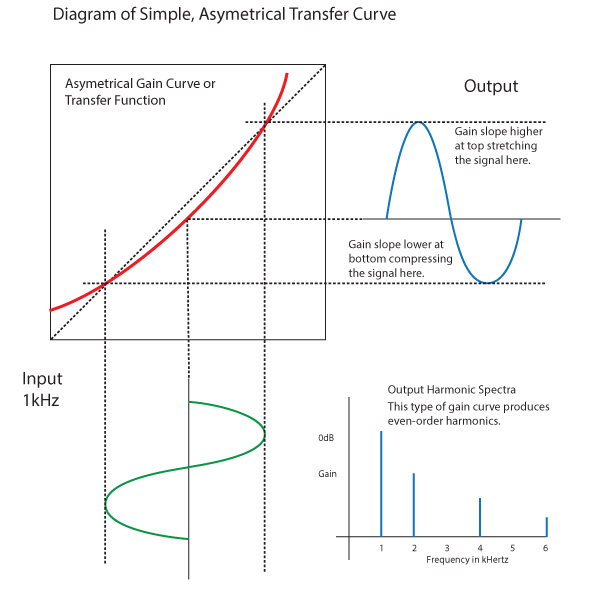
An asymmetrical transfer curve has different gain profiles between the positive and negative going portions of the waveform.
In the above plot we see a simple "C"-shaped curve as the transfer curve. This curve will produce more gain (steeper slope) for the positive half of the incoming waveform than it does for the negative half (less slope). This will result in the positive half of the output waveform being stretched and the negative half being squished. This type of distortion will produce even-order harmonics, and you can see in the harmonic spectra plot 2kHz, 4kHz, and 6kHz harmonics are being created from the probe tone.
This type of distortion is often seen in single-ended, class-A amplifiers with single output devices. It can also occur in headphone when there are asymmetrical forces at play. For example, there is a limited amount of acoustic space behind the driver. As the driver moves outward away from the structure behind the diaphragm they have less effect than when the driver moves inward toward the structures. This produces an asymmetry in response between the compression and rarefaction stroke of the driver.
Another asymmetrical phenomena exists due to the diaphragm being firmly fixed at its edges (for most dynamic headphone diaphragms), which causes the useful driving surface of the diaphragm to get smaller as the diaphragm moves away from center. But because of the bulging shape of the taurus between the fixed edge and internal dome, the change in driving area with excursion is different depending on whether it's moving outward or inward.
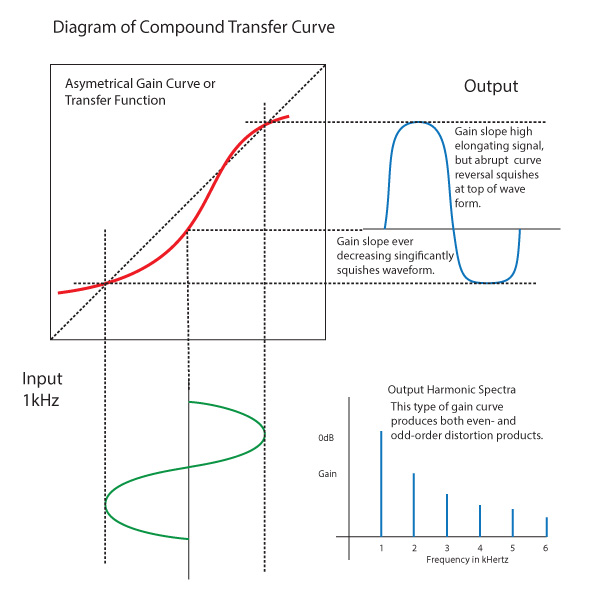
Most system will exhibit some amount of both symmetrical and asymmetrical bent in its transfer curve.
The truth is most systems will exhibit some amount of both symmetrical and asymmetrical behavior and will produce both even and odd harmonics. In fact, it's been suggested that when looking at the harmonic series, the best sounding products will exhibit both even and odd harmonics and they will appear in nice, smooth, ever decreasing series. Unfortunately, InnerFidelity's THD+noise measurement is unable to show this.
Harmonic Distortion Summary
All the above dialog about the shape of the transfer curve of the device under test and how, when not linear, it will produce harmonic overtones fall into the "THD" part of the THD+noise measurement. Put in a pure 1kHz tone, and you'll get some of that energy moved into a higher frequency that is a multiple of the original probe tone.
However, there are other mechanisms that might cause probe tone energy to be moved into other frequencies that have nothing to do with the transfer curve of the device under test. These spuria fall under the heading of "noise" in the measurement.
Noise Sources in THD+noise Measurements
Many headphone enthusiasts have experienced the dreaded "hair in the driver" syndrome. This is where a hair works it's way through the various coverings in front of the drive and is beginning to touch the diaphragm as it moves causing a buzzing noise—very bothersome if you've ever experienced it. The thing about this buzz is that it creates a broad band noise that isn't limited to the harmonic structure of the probe tone—it is a noise source and is measured by the THD+noise measurement.
Another example of a noise source might be if a small part is loose and rattles. In this case, the rattling might be frequency sensitive: at 100Hz the part might rattle, but at 1kHz the probe tone frequency might be too high to stimulate the rattle. The THD+noise measurement will show this as elevated distortion at those frequencies where the rattle occurs.
A third example, and one that is very important with headphone measurements is the problem of diaphragm break up, which usually occurs at frequencies above 1kHz. Diaphragm break up happens when the normal pistonic movement of the diaphragm moving forward and back begins to exhibit another type of movement—sometimes rocking motions, sometimes folding motions (think taco) of the diaphragm. These oscillatory mode of the diaphragm movement will produce tones in addition to the probe tone. They will be mathematically related to the probe tone, but won't necessarily be in the harmonic series. None the less, they will be measured and will appear as features on the THD+noise plot.
Power Handling and THD+noise Plots at 90dBspl and 100dBspl
The last thing to note about THD+noise measurements at InnerFidelity is that the THD+noise measurement is done at two different sound pressure levels in the headphones: 90dBspl and 100dBspl. Most people consider about 85dBspl as a reference listening level—if you're going to mix a record, you should do it at about 85dB. It's a pretty solid level, and louder than I normally listen for enjoyment. So, the 90dBspl THD+noise plot is fairly indicative of the worst case amount of distortion you'd get during normal listening. But, we have to remember that there will be dynamic peaks in the music much louder than the average level, so it is reasonable to test for distortion at higher levels, which is why InnerFidelity measures THD+noise at 100dBspl as well.
The thing to know about the THD+noise plot is that it is the amount of signal present apart from the probe tone measured relative to the amplitude of the probe tone itself. If I measure 1% THD+noise at 1kHz at 90dBspl, and the same 1% at 100dBspl, there will actually be 10dB more THD+Noise in the second measurement because it's measured relative to the 10dB higher in level probe tone.
Most headphones will exhibit mildly worse THD+noise numbers at higher volume levels, but some will exhibit much worse figures at some frequencies as the level goes from 90dBspl to 100dBspl. In that case we can say the headphone has poor power handeling, and is on the ragged edge of misbehavior during the high volume peaks of the music.
Conversely, we can sometimes see headphones where the 100dBspl THD+noise plot is below the 90dBspl plot. In this case we've got a headphone that is very well behaved as volume gets louder and we can say the headphone has good power handling capability.
THD+noise Plot Summary
The THD+noise plot sweeps a probe tone from 20Hz to 7kHz through he device under test. This probe tone will stimulate various distortion mechanism in the device under test, which will move some of the probe tone energy elsewhere in the frequency spectrum. The resulting signal is sent to an audio analyzer that first filters out the probe tone with a narrow notch filter that tracks the probe tone as it is stepped through the spectrum. The audio analyzer then measures the RMS amplitude of the remaining signal, which contains all the total harmonic distortion and noise products of the probe tone.
Maybe the most important thing to know about my THD+noise measurements is that they're the most likely plot to be erroneous. Because it's a very sensitive acoustic measurement and I don't have a laboratory grade isolation chamber, if a large truck goes down my street during a THD+noise measurement you'll probably see it in the plot as a small rise. Also, if water is running in my house or if the refrigerator kicks on, these might produce enough noise to increase the recorded THD+noise. Lastly, for about six months last year I was having some odd symptoms with my Audio Precision tester—it took a while for me to even realize I had a problem—and it does seem that it effected some of the THD+noise measurement. The AP tester is fixed now, and THD plots do seem more stable.
There are two spikes at 200Hz and 2kHz in THD in all plots, this is an artifact of the tester changing ranges at those frequencies. These can be ignored.
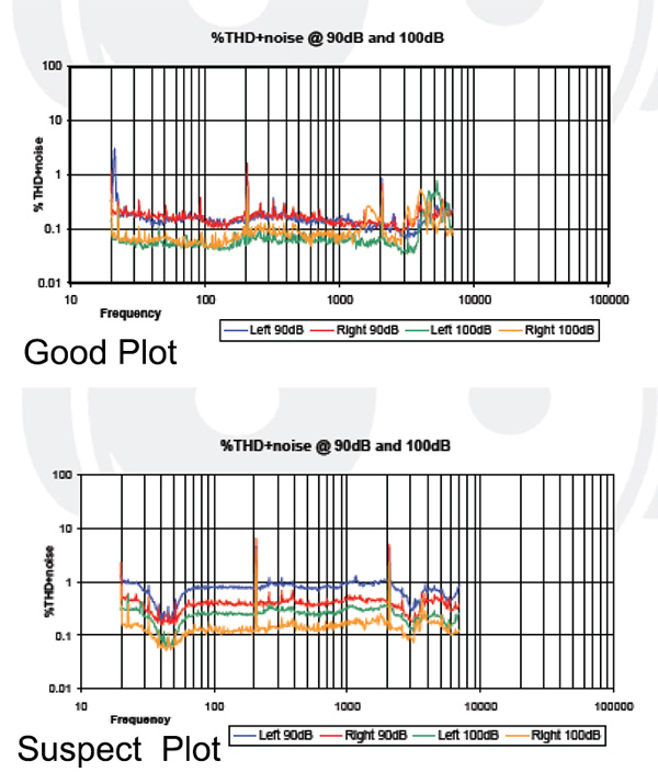
My point is that THD+noise plots should be taken with a big grain of salt. Here's the kind of thing you're looking for to determine if a feature of a THD+noise plot is real or not. In the top good plot above, you'll see that the average level of the 90dB plots (red and blue) is just above the 0.1% line and the 100dBspl plot (yellow and green) is just under the 0.1% line. This is probably near the noise limit of my system, so the headphones measured may actually be lower distortion than indicated.
On the yellow line of the top plot between 1500Hz and 2kHz you'll see a bump that doesn't exist in the green plot. My THD+noise plots are taken one channel at a time, is quite possible that this is just a truck going down my street. However, above 3kHz you can see both the yellow and green line becoming noisy and a little more elevated; because both channels are doing it and because the rest of the plot is quite low, I suspect there is a real rise in THD above 3kHz here. As a rule of thumb, 1% is considered the point at which distortion becomes a problem.
In the bottom suspect plot above, you can see that all four plots have near the same shape and relatively low levels of noise. Left and right channels are offset but of similar shape. I suspect there's something wrong with this plot due to the problem with the AP tester.
Bottom line here: Don't worry too much about small features on the THD+noise plots; it's the larger features that are most telling. Let's have a look at them.
Distortion Rise in Bass
As the frequency gets lower and lower headphones will often have a harder and harder time reproducing the long wave form faithfully. My current working theory is that in open headphones it happens because the driver goes below its primary resonance and begins to be unable to properly track the waveform or begins to hit its physical movement limits. In sealed and on-ear headphones it generally happens when you reach a limit of how much pressure can be contained in the chamber between the ear and the driver, and the waveform begins to soft-clip.
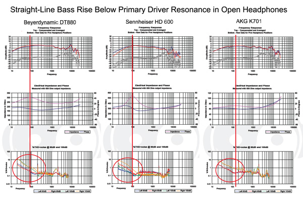
The plots above are three different dynamic, open, circumaural headphones. The red lines are positioned at the primary driver resonance, which is indicated by the peak in the impedance plots (center row of graphs). You can see in the frequency plots at the top of the image that this is the point at which the bass starts to roll off. You can also see that it is generally just above this frequency that the rise in THD+noise begins. Notice on all threeTHD+noise plots this is a straight line. This is very common, though not optimal, behavior for dynamic open headphones.
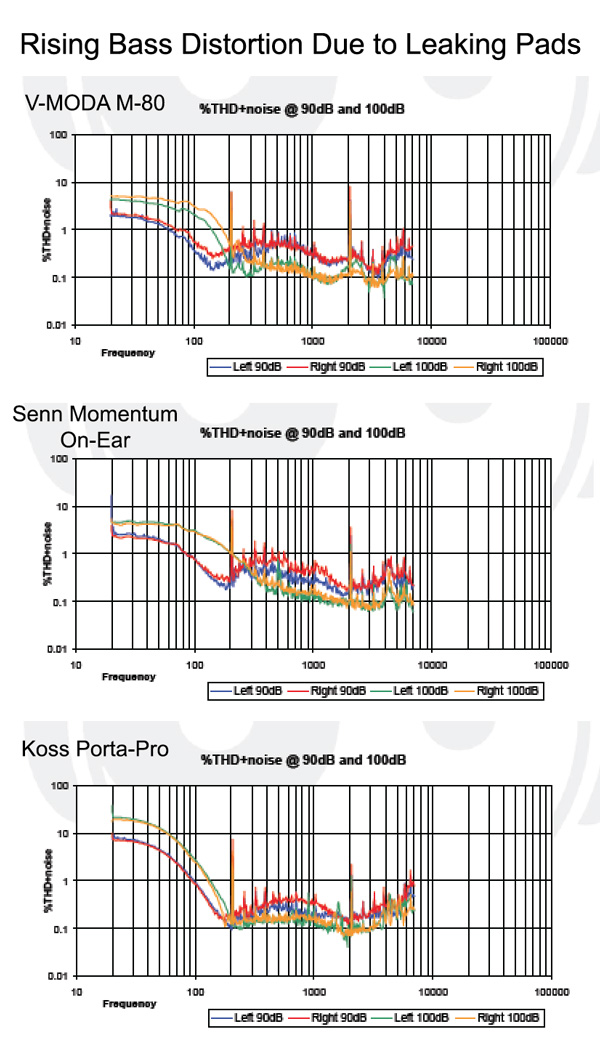
The other kind of bass distortion I see is a curved rise in THD, which I think comes from a limitation of how well the ear pad is holding pressure at low frequencies. It's often seen in on-ear type headphones, but it can be observed with most headphone types.
Both types of rising distortion in the bass are audible and generally impart a loose, wooly sound depending on the magnitude of distortion. Headphones without the bass distortion are likely to sound tight and punchy in comparison.
Distortion Peaks
Another feature to be seen in the THD+noise plots are peaks both wide and narrow. These peaks arrise usually due to resonances or diaphragm modal break-up.
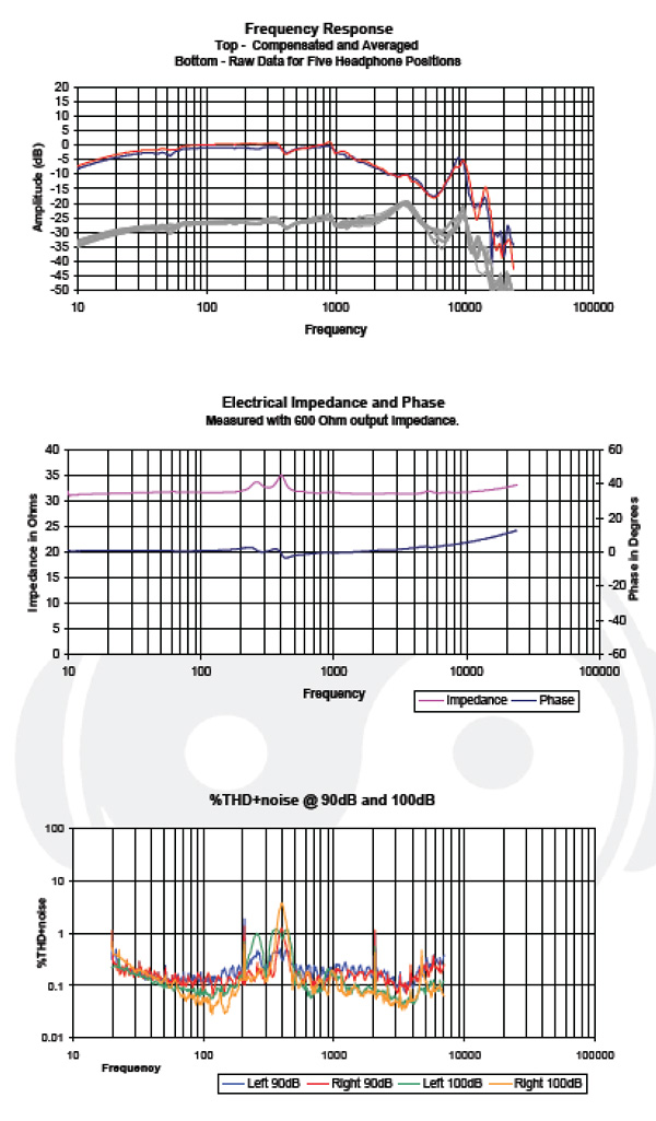
When interpreting THD+noise it's a good idea to look for related features on the impedance and frequency response plots for clues to the nature of the peak. The plot above is an Oppo PM-1. You'll notice it has elevated THD between 200Hz and 500Hz. You can also see that it has a couple of bumps in it's impedance in that area, as well as some wiggles in its frequency response there. What we're seeing is a pair of diaphragm resonances from the just the central part, and then the whole diaphragm surface. The magnitude of the distortion is just 1% at 100dBspl—which is pretty looud—so I would consider this a minor problem for these headphones.

The AKG K812 shown above is a good example of something being quite obviously wrong. We can see a clear rise in THD between 1kHz and 3kHz, and we can see some associated wiggles at those frequencies in the impedance plot. Generally speaking, the impedance plot should be smooth and relatively featureless. It's okay to have a fairly large hump from the primary driver resonance, and there are usually some small bumps in the 2-6kHz area from resonant spaces around and behind the driver, but the curve should look smooth and regular overall.
On the above AKG K812 impedance curve you can see that the bumps and wiggles starting at 1.5kHz are rather irregular shaped. This is not a good sign and coupled with the broad rise in distortion indicates some significant driver problem in this area, possibly modal break-up of the diaphragm. That the distortion only just surpasses 1%—and not taking into consideration other plots for this headphone—is an indicator this problem may be modest.
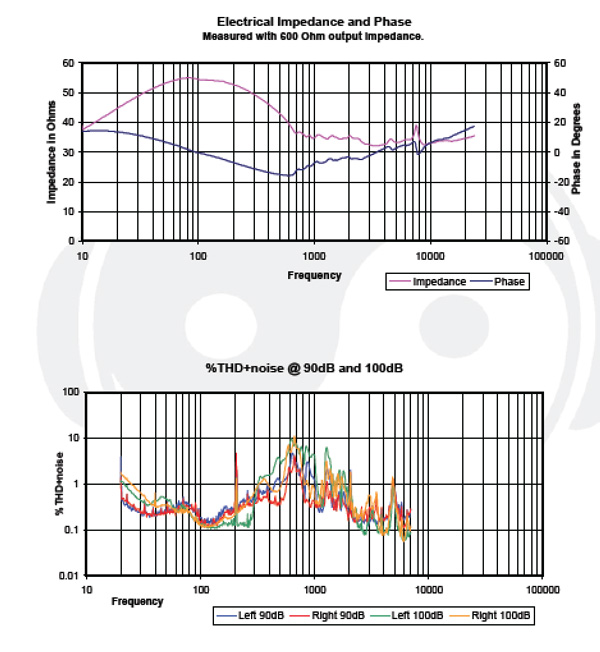
On the other hand, here is a plot of the Beyerdynamic T5p and we can clearly see distortion exceeding 1% even at 90dB, and reaching 10% at 600Hz at 100dB. The associated impedance plot is also extremely irregular. This headphone would be expected to sound very hard through the mid-range.
 Unlike the broad bump increase in the previously discussed headphones, the Skullcandy Grind, shown above, exhibits three distinct narrow peaks in the THD+noise response at about 1.6kHz, 2.1kHz, and 3.7kHz, and relatively small and regular related features on the impedance plot. This leads me to believe these are resonances in the space behind the driver rather than modal break-up, and even though the THD peaks exceed 1% at 100dB, this symptom is less damaging to the sound quality than the previous two headphones.
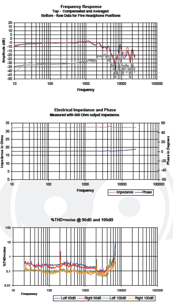 The last headphone we'll check out for a distortion peak is the Audeze EL-8 above. The THD+noise plot look really, really good...until you get to 4kHz where it starts to rise significantly. The impedance plot appears unchanged, however. These are planar magnetic headphones, which will often times not exhibit changes to impedance with resonance problems. But, if you look at the frequency response plot, you will see a very large dip in response centered at 7kHz that's likely due to a resonance of some type. The rise at the very end of the distortion plot is very likely related to the dip in frequency response.
Power Handeling
THD+noise sweeps are done at both 90dBspl and 100dBspl. When the 100dBspl sweep is plotted, the increased volume improves the systems signal to noise ratio, and because THD+noise includes a noise component, the result can be a lower measured value at higher volumes...as long as the headphones aren't increasing in distortion at the higher volume.
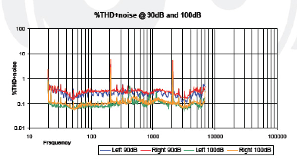 Above is the THD+noise plot from an Audeze LCD-2. The entire 100dBspl plot (green and yellow) lies below the 90dBspl plot (red and blue). This means that even though the headphone is being played quite a bit louder there is very little increase in distortion otherwise it wouldn't have remained under the 90dBspl plot. This headphone has good power handling; it can be played loud without distorting.
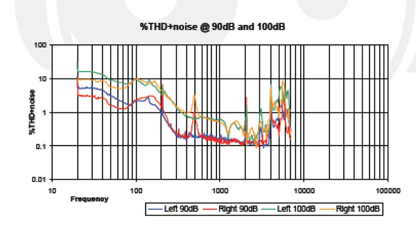
The Ultrasone HFI-450, on the other hand, shows the 100dBspl plot significantly above the 90dBspl plot indicating it is increasing in distortion significantly as volume increases. This headphone has poor power handeling.
THD+noise Examples Summary
THD+noise plots are the measurement most prone to error in the InnerFidelity headphone measurement spreadsheets. Be careful not to over-interpret small features that may be cause by environmental noise during the measurement and not the headphones.
THD+noise plots are good at identifying three things:
- Rising distortion in the bass due to the driver running out of steam when it goes below its primary resonance, or due to leaky pads that can't retain the pressure needed for low frequencies.
- Distortion peaks due to resonances and diaphragm break-up. These features are usually accompanied by features in the impedance and frequency response curves that can help you determine what kind of problem is in evidence.
- Because THD+noise is measured at both 90dBspl and 100dBspl, it is possible to see if distortion is rapidly increasing with volume or not, which will indicate whether the headphone has good power handling or not. As a general rule: the more the 100dBspl plot is below the 90dBspl plot, the better power handling it has.
Electrical Impedance and Phase
Introduction
The fundamental DC resistance in a pair of headphones is primarily due to the length and thinness of the wires in the voice coil of the driver. The longer and/or thinner the wire, the more resistance it has. This resistance is a constant and will not change with the frequency of the applied signal.
In this article, we're primarily going to discuss the reactive nature of the headphone driver as an electrical load on the amplifier driving it, which is expressed as impedance and is essentially additive to the resistance of the voice coil. Impedance is somewhat like resistance in that it can be expressed in Ohms, but it's quite different in that it is "reactive" and the impedance in Ohms can change depending on the frequency applied. Here's how that happens.
Imagine a pendulum that swings at a rate of once per second or 1Hz (its natural resonant frequency). We now mount a motor on it and drive the motor with a 1Hz signal. Because this is the resonant frequency of the pendulum the motor doesn't have to do much work; it only needs to add enough energy to prevent the decay of the swinging motion.
Now imagine we try to send the motor a signal to drive the pendulum a little slower at 0.8Hz. In this case, the pendulum will always be fighting to go a little faster than the drive signal, and the amplifier driving the motor will have to resist being drug ahead to the faster natural rate of the pendulum. Remember, the motor is also an electrical generator, and the pendulum wanting to swing ahead of the drive signal will create its own reactive electrical motive force that the amplifier will have to damp in order to maintain the desired signal.
This is the fundamental difference between resistive and reactive loads: in resistive loads the impedance remains constant; in reactive loads, the load will "fight back" by producing back EMF (electro motive force) that will vary depending on the frequency.
Now imagine we try to drive the pendulum at 1.2Hz—faster than its natural resonant frequency. In this case, the pendulum will fight to slow down, and the amplifier will have to apply more voltage to overcome the pendulums effort to retard the drive signal.
Looking at the Sennheiser HD 580 electrical impedance and phase plot above, we can see the driver's primary resonance on the impedance plot (purple line) as a large peak centered at about 90Hz. This is analogous to the natural swinging rate of the pendulum discussed above.
You can also see the electrical phase, (blue line) starting at the left at 10Hz, slowly advancing in phase (rising on the plot; phase axis labels in degrees shown on right) more and more as it moves higher in frequency towards the resonance. This advancing phase is due to the driver resonance "pulling" the electrical signal towards resonance—similar to when the pendulum pulled towards resonance when we tried to drive it at a slower rate.
As we go through resonance at 90Hz and beyond, we see the phase swing through zero and go negative above resonance. This is due to the driver back EMF fighting against the drive signal and trying to retard it back toward the resonant frequency.
The bottom line here is that as we approach the resonant frequency of the driver from above or below, it fights harder and harder against the amplifier by generating its own counter EMF, making the impedance go higher as we near resonance. At resonance, the driver is most efficiently creating its own EMF, and therefor has its highest impedance to change. This is a little counter-intuitive as this is also the point at which the driving amplifier has the easiest job powering the driver, but remember, it's also the most difficult place for the amplifier to drive the driver away from, and therefore has the highest impedance.
In other words: There is a very close relationship between the impedance and phase plots...so close, that you usually don't need to bother looking at the phase plot as what information can be gleaned from this data is usually available in the impedance plot.
ELI the ICEman
This is a little mnemonic used in basic electronics education to help remember the relationship between voltage and current in a reactive system. The letter E is for voltage, and I is for current; the L is for inductive loads, and the C is for capacitive loads. The mnemonic reminds us that voltage leads current in inductive loads, and current leads voltage in capacitive loads.
In the HD 580 phase plot above (blue line) you can see that the electrical phase angle at 40Hz is advanced about 8 degrees. Because voltage is leading, in this case, we can say the amplifier is seeing an inductive load at 40Hz. At 200Hz, the electrical phase angle is about -7 degrees. Because the electrical signal is lagging behind, we can say the amplifier is seeing a capacitive load at 200Hz.
The voice coil itself is an inductor, but inductors of this size are relatively ineffectual at low frequencies, but can begin to exert its reactance as frequency gets higher. Turning our attention to the right hand side of the plot, we can see that both the impedance and phase angle start slowly rising as frequency gets higher and higher. This is the reactance of the voice coil acting as an inductor coming into play.
Virtually all voice coil (normally called dynamic) drivers will exhibit this slow inductive rise in the high frequencies. Planar magnetic headphones typically do not have coils but rather serpentine driver traces on their diaphragms. Since they are not a coil of wire they are not very inductive, and they do not exhibit this rise in impedance and phase at high frequencies. The one exception is the Oppo brand of planar magnetics, which have a circular pattern of diaphragm traces which do act as an inductor. As we will see later in this article, they do have this slowly rising impedance and phase at high frequencies.
Other Sources of Reactance Indicated in Impedance and Phase
As we've seen, the primary driver resonance creates back EMF that changes the impedance and phase characteristics measured. But there are other sources of resonance and reactivity of headphones that can be seen in the impedance and phase plots.
Many acoustic resonances in the headphone can exert acoustic back pressure on the driver, which will, in turn, be converted to an electrical back EMF which can be sensed in measurements. These can be high frequency resonances in the small areas near and within the driver, or they can be lower frequency resonances in the ear capsule behind the driver, and in the enclosed space between the driver and the ear.
Another source of reactance is the crossover networks of multiple balanced armature IEMs and in hybrid, dual-drive headphones.
Okay, let's take a closer look at some plots.
Impedance and Phase Plot Interpretation
Let's start with a well behaved, open acoustic headphone. I'll repost the HD 580 from the top of the page here:
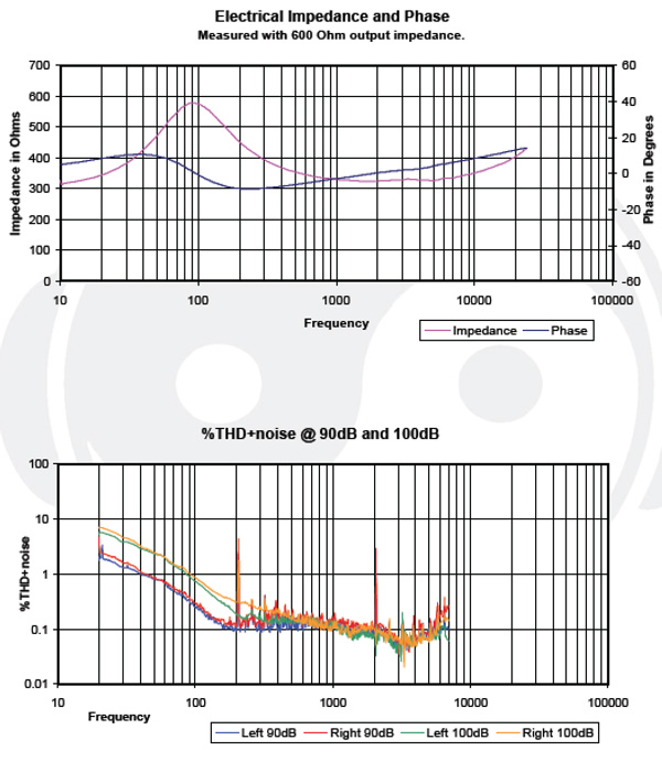
In open headphone designs, the driver sees very little acoustic damping as it's essentially suspended in free air, which allows it to move without restriction. Almost all open headphones will show a primary driver resonance somewhere in the 60Hz to 150Hz range. The amplitude and narrowness (Q) of this peak can vary widely, however.
Also note that other than the resonant peak and slowly rising response in high frequencies there is very little other features on the plot. This is a good thing; it means that there are few other resonances in the headphone to disturb sonic performance. Also note that the distortion plot (THD+noise) shows very few features pointing to poor performance. It does, however, show rising distortion in the low frequencies in part related to the amplifier having to work hard to drive the load below its resonant frequency.
Sealed Headphones
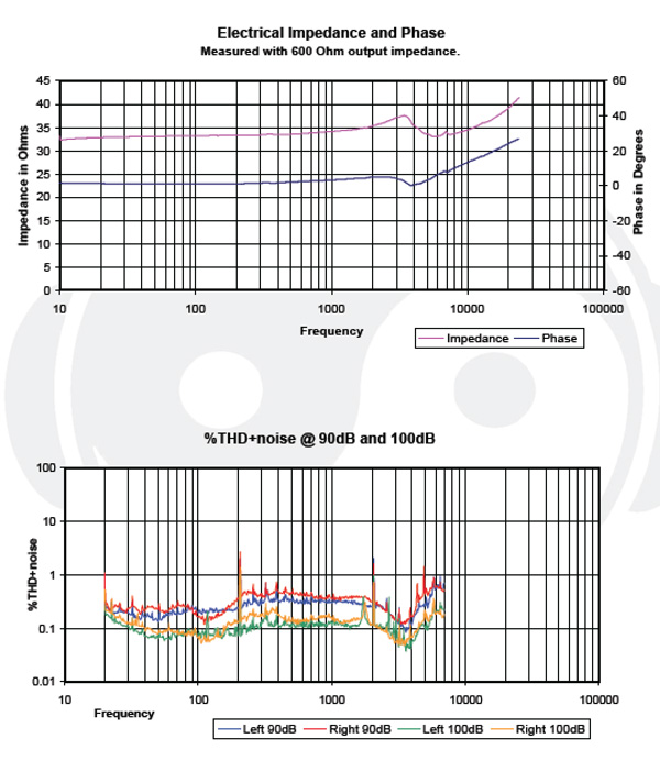
Plots for the Focal Spirit Professional.
The Focal Spirit Professional shown above is a sealed headphone. In sealed headphones, acoustic damping can act to reduce or eliminate the primary driver resonance. Here we see that in the FSP. There does appear to be a resonance at 3.5kHz, but there is no increase in distortion at that frequency, so this resonance is likely by design. Looking at the FSP measurement data sheet, we can see that there is a rise in frequency response corresponding to this impedance peak. It's very likely this resonance was created to shape the frequency response to have a peak at 3.5kHz, which is desirable as described in the Harman Target Response curve.
Back EMF from Pad Bounce
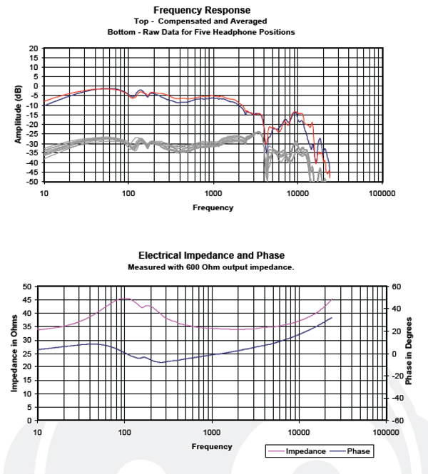
Sennheiser HD 449, a low-cost, circumaural, sealed headphone.
"Pad Bounce" is a term I use to describe the phenomena of a resonance born from the springiness of the ear pads and enclosed air between the driver and ear. Many headphones have pad bounce, but inexpensive headphones using cheap, springy foam (not memory foam) are quite likely to exhibit the behavior.
In the frequency response plots of the Sennheiser HD 449 shown above, you can see some strong wiggles between 100Hz and 200Hz from a pad bounce resonance. Unusually, you can also see a coincident feature in the impedance and phase plots at about 170Hz. Essentially, the acoustic feedback from this pad bounce is impressing itself on the driver's movement and changing its impedance at the resonance. In my experience, pad bounce doesn't affect the listening experience much.
Planar Magnetic Headphones
As mentioned earlier, typically, planar magnetic headphones do not have a voice coil but rather a serpentine layout of traces on the diaphragm surface. As such, planar magnetic headphones are almost purely restive in nature, and have little reactive properties when driven.
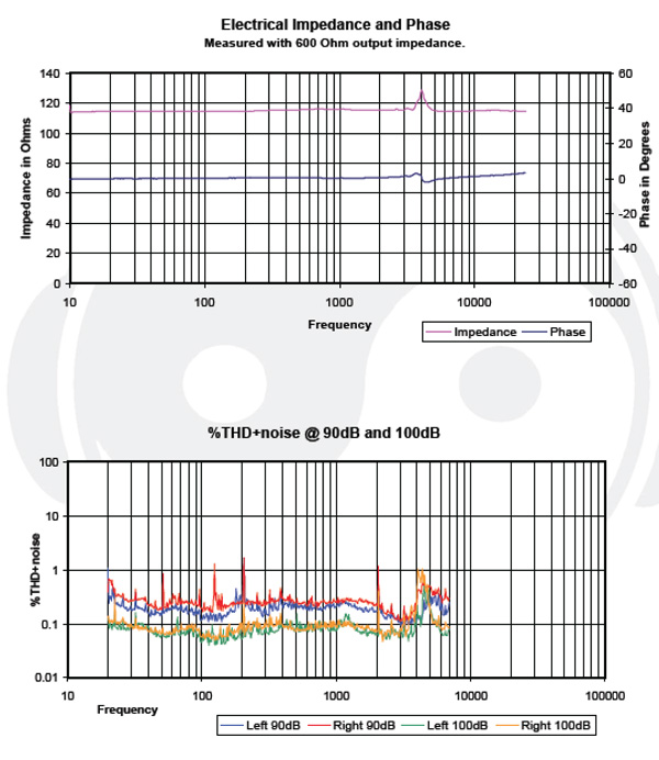
Audeze LCD-3 planar magnetic headphone.
In the Audeze LCD-3 plot above, you can see that the impedance plot is nearly ruler flat at about 115 Ohms. This is typical of planar magnetic headphones.
You can also see a small but distinct feature at 5-6kHz on both plots. Because of its high frequency, this resonance is likely confined in a small space in the driver, somewhere close to the magnets and diaphragm. The thing to note here is that there is a corresponding distortion increase at this frequency.
Here's another LCD-3 plot.
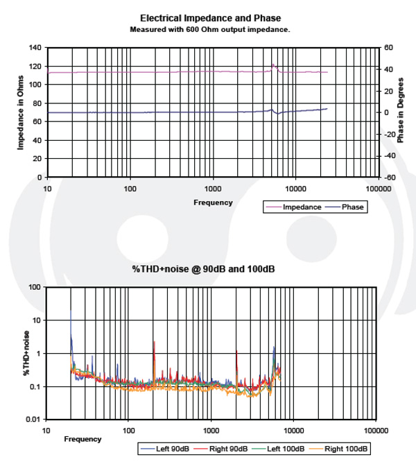
In this plot, you can see the feature in the treble is now at 4kHz, and the corresponding peak in distortion has moved lower in frequency as well. It's interesting to note here that this feature on LCD series cans is much more apparent on models with the Fazor, with the notable exception of the LCD-4 which has a Fazor but no feature at this frequency.
My point here is that it is sometimes possible to relate features on the impedance and phase plots with spikes in distortion. It may or may not have audible effects, but I have to feel that it tends to indicate a design that could be improved upon.
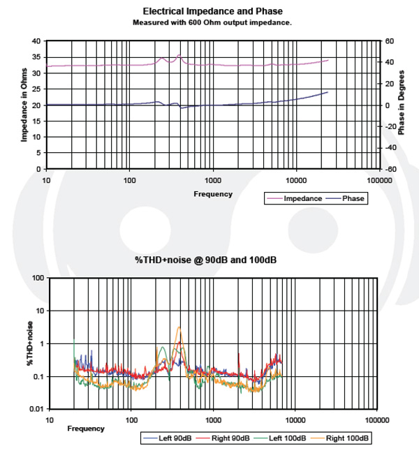
Oppo PM-1 planar magnetic with coiled traces.
The Oppo PM-1 shown above has coiled diaphragm traces as opposed to the serpentine pattern of most planar magnetic headphones. As such, it does behave a little like dynamic headphones with voice coils, which can be seen in the slowly rising impedance/phase response in the high frequencies as it begins to act like an inductor.
Also, you can see two resonant humps in the impedance at 250Hz and 400Hz. I was told by Oppo that these are the primary driver resonance peaks—one from the center area of the driver, and the other from around the edge area of the driver. Two corresponding peaks in distortion can also be observed.
Impedance Plots Give a Peak at Driver Design Quality
Though headphones are far too complex to closely diagnose problems from InnerFidelity impedance, phase, and distortion measurements, I do find they give a general sense of how well a driver is designed. As mentioned previously, excessive and rough bumps and wiggles in the 2-7kHz region may be evidence of poorly designed acoustics in the small spaces near and inside the driver assembly. The following plots show a clear relationship between rough spots in the impedance and phase plots at 2-7kHz and increases in distortion.
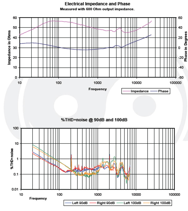
AKG K812.
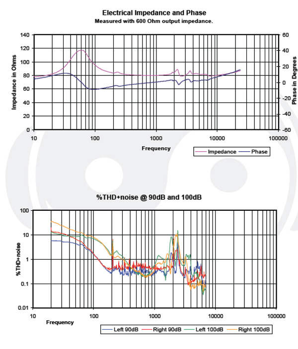
Ultrasone HFi 2400.
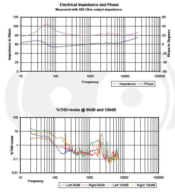
Ultrasone Pro 650.
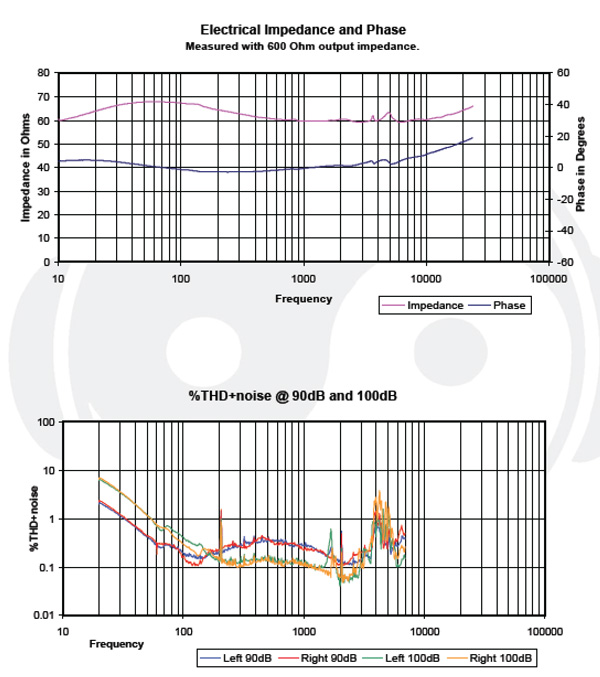
Takstar Pro 80.
In all the above cases, I heard a significant roughness to the response likely due to acoustic problems in and around the driver.
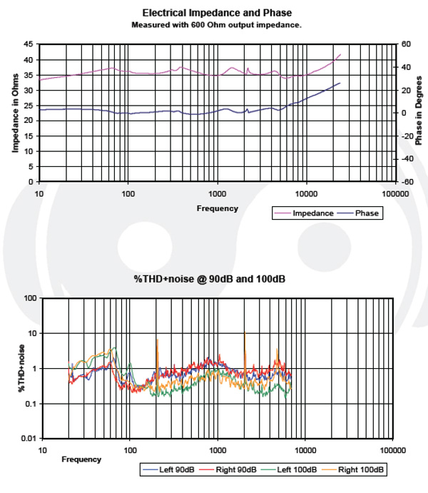
California Headphones Silverado.
Things are not always so simple however, the above California Headphones Silverado shows a very uneven impedance response, but no apparent relating peaks in distortion—though overall distortion is a bit high. In this case, a look at the entire measurement .pdf does show a significantly uneven frequency response, with feature that do coincide with impedance response features. This headphone simply has poorly designed acoustics broadly, and sounds quite colored with numerous internal resonances probably coming from a variety of sources.
Making the peak at 3.5kHz in IEMs with a resonance.
The concha bowl of your ear creates a resonance at about 3.5kHz that shows up on raw frequency response plots, and is needed for you to perceive the sound as flat through that range. When wearing regular headphones, this peak in response naturally happens because the sound is coming through the concha area in a way similar to normal sound.
But once an IEM is inserted into your ear canal, the concha is acoustically bypassed. IEM makers then need to find a way to artificially produce the peak at 3.5kHz. This is typically accomplished by designing the driver such that it has a natural resonance at 3.5kHz and will then therefore produce the desired peak in frequency response.
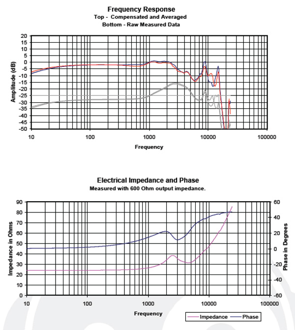
Etymotic ER4PT
The plot above shows the Etymotic ER4PT single balanced armature IEM. You can see there is a feature in the impedance plot in the 2-4kHz region indicating a resonance there. This resonance is designed to provide in increased frequency response, which you can see in the raw frequency response plots as a lovely gentle hump at about 3kHz. Many IEMs, both balanced armature and dynamic driver, will show a resonance in the impedance plot for this purpose. A nifty trick!
Non-Acoustic Sources of Impedance and Phase Response Features
Multiple Drivers - Variations in impedance can occur for reasons other than acoustic resonances. Headphones with multiple drivers will exhibit fluctuations in impedance both from the differing resonances of the various drivers, and from the reactive components (inductors and capacitors) of the cross-over components. Let's take a look at some multi-balanced armature driver IEMs.
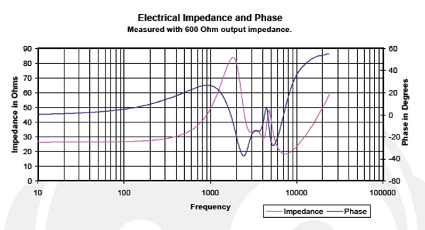
V-Sonic VC1000.
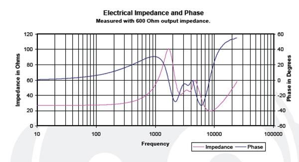
Phiaton PS200.
The two sets of plots above are dual-balanced armature IEMs. You can see that the impedance plot is quite complex. I've stared for a long time at multi-BA IEMs and I can tell you that it's not readily apparent from the plots how many drivers are in the IEM. None the less, these are quite obviously more complex impedance plots than the Etymotic ER4PT single BA driver IEM shown above. How about 3 BA drivers?
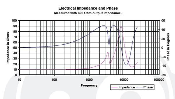
Sony XBA 3iP.
Even though the Sony XBA 3iP has an additional driver, it's plots do not look more complex than the two dual BA IEMs above. I assume the complexity of multiple drivers and crossover components make it quite difficult to clearly determine the number of drivers from the impedance plots unless you're quite expert at IEM design.
It's also worth noting at this point that multi BA IEMs can have very large swings in impedance. For example, in the Sony XBA 3iP above, impedance can vary between 10 and 100 Ohms. This can be a big problem if your headphone amplifier has a high output impedance.
Let's say the output impedance of your amplifier is 10 Ohms. With the Sony XBA 3iP, the impedance below 1kHz is about 10 Ohms. That means half the amplifier's voltage will be dropped across the output impedance of the amp, with the other half of the voltage going to drive the headphones. At 8kHz the Sony has 100 Ohms impedance—ten times that of the output impedance of the amp. Now, only about 1/10th of the voltage will be dropped across the amplifiers output impedance, while the other 90% will be available to drive the headphones. In other words, with a high output impedance amp and low, but swinging impedance headphones, as the impedance of the headphone rises, the drive voltage to the headphones will rise. This causes the frequency response of the headphones to vary along with the impedance curve.
Bottom line: if you've got multi-balanced armature IEMs, make double-damned sure you've got a low output impedance amplifier to drive them or you'll end up with a colored listening experience.
Multiple drivers can also be found in regular sized headphones, and will exhibit similar features in their impedance and phase response.
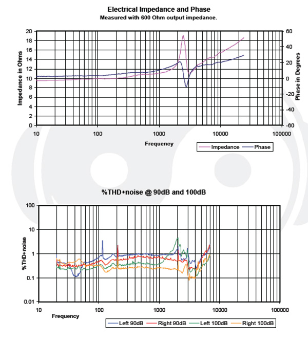
Final Audio Pandora Hope 4.
The above plot of the Final Audio Pandora Hope 4 headphone is a hybrid dynamic/balanced armature headphone. I'm not aware of what components exactly are inside, but it's fairly obvious that something is going on 2-3kHz, likely the cross-over point of the headphone.
Other Oddities
And lastly, a couple of odd things you might see perusing InnerFidelity impedance response plots.
Other Components in Circuit - The Audeze SINE is a planar magnetic headphone, and as such ought to have a fairly flat impedance response. As you can see below, there's a significant feature at about 2.5kHz in the impedance/phase response, but no corresponding increase in distortion (in fact, distortion reduces there).
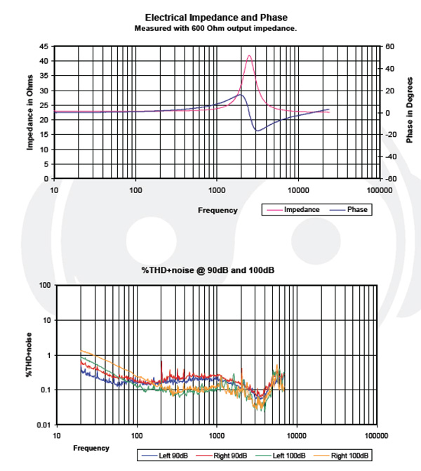
Audeze SINE.
This feature comes from a small resonant circuit (an inductor and capacitor) used to surpress a peak that would otherwise appear in the frequency response. This small reactive circuit can clearly be seen in the impedance plot.
Active Circuits in Headphones - Many headphones have active electronic circuits in the headphone for bass enhancement or noise canceling. In this case, one often sees very high impedances as the incoming signal is no longer being applied directly to a driver, but is now seeing the input of an electronic circuit—which is often quite high.
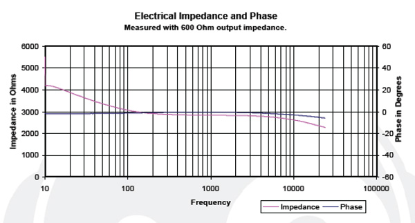
Bose Quiet Comfort 20.
The above shown Bose Quiet Comfort 20 is a noise canceling headphone with the electronics activated. The input impedance to these headphones is around 3000 Ohms in this mode. The impedance rise in the bass may be evidence of capacitive coupling on the input to the analog circuits.
Square Wave Response
Read about square waves and the most common thing you'll hear is they are made of a fundamental and an infinite set of odd harmonic tones in a very particular amplitude and phase relationship. That's true, of course, but in the real world and with regard to testing headphones, it may not be the best way to think about them. It's a decent place to start though.
Viewing Square Waves as Made of a Fundamental and Odd Harmonic Series
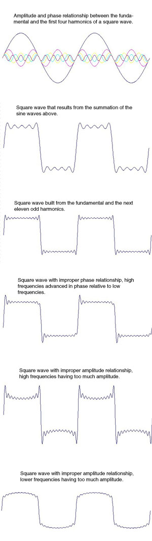 To show you how square waves are built from a fundamental tone and its odd harmonics, I created a little Excel spreadsheet. In the spreadsheet (you can download the Excel file here). I used some simple math to create a series of columns holding data that represented the appropriate sine waves that I could then add together to form the square wave. The formulas used also had some variables with which I could control the relative amplitude and phase of the odd harmonics.
The top plot to the left shows the fundamental tone and the first four odd harmonics. The next plot shows the result of simply adding together the amplitude of the signals at each point in time. You can see clearly that the result begins to look quite like a square wave. The third plot shows the result using the first 11 odd harmonics, and you can see does a better job of making a facsimile of a perfect square wave. As more and more odd harmonics are used, the square wave gets closer and closer to the ideal. In band width limited systems--like a DAC that might have a limit of 22kHz for 16/44 CD playback--only a limited amount of odd harmonics available, and square wave reproduction will look quite like the third plot.
There are two other things that can misshape the square wave response: phase and relative amplitude errors between the fundamental and harmonics. In the fourth plot, the phase (time relationship) of the odd harmonics is advanced as the frequency gets higher. In audio electronics gear, all frequencies are delayed a little, but high frequencies typically move through the circuits a little more quickly than low frequencies. The words "group delay" are used to identify this phenomenon. Group delay creates phase error in the timing relationship of all the odd harmonics of a square wave. In the fourth plot to the left, I've introduced some phase error, and you can see how it changed the shape of the square wave some and introduced an overshoot on the leading edge.
Errors in the amplitude relationship of all the odd harmonics can occur if the system's frequency response is not flat. In the second to last plot at the left, I've simulated a tipped-up frequency response (less bass, more treble), and in the last plot I've simulated the opposite with more bass and less treble.
This is a valid way to look at square waves for some applications, but it makes some assumptions about the sine waves being continuous forever that make it a little misleading in terms of the type of square wave testing I do on headphones. For example, in the third plot down, you can see little spikes before the transitions. This is called "pre-ringing." How could an analog system know the signal is about to change and create the pre-ring? Answer: it can't. That's one of the reasons why it's better to look at square wave response as a series of step responses.
Step Response and Square Wave Response
Step response is simply measuring how the device under test responds to an instantaneous shift in level. From 0Volts to 1Volt, for example. As long as the frequency of the square wave used is longer than the lowest frequency of interest, a square wave is simply a series of step responses.
Step response is used broadly in audio electronics and electronics in general to indicate a variety of performance characteristics in the time domain, such as rise time, overshoot, settling time, and ringing. But step response also contains phase and frequency response information. For example, it is one of the speaker characteristics John Atkinson measures to look at the phase coherence of a multi-driver speaker. (His very interesting explanation is here.)
You can also think of step response as a measure of frequency response where the leading edge slew rate indicates the high-frequency limit, and the length of time it can keep the step at the new level an indication of its low-frequency limit. At every point between, you can think of the level of the top of the step response as related to the frequency response at the frequency whose quarter wavelength is equal to the elapsed time since the leading edge of the step/square wave.
Another way to look at it is similar to the summation of a series of odd harmonics we talked about above. You can think of a step response as the amplitude response of a continuous series of equal amplitude narrow-band pulses.
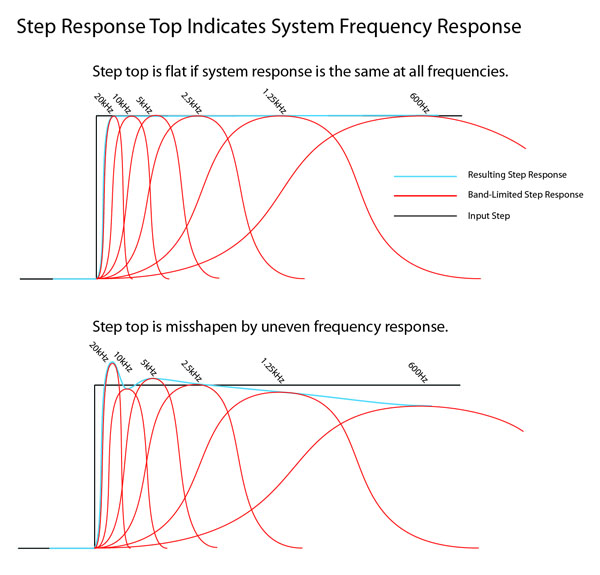
This graphic illustrates the idea that the step response can, in part, be thought of as the plot of amplitude maxima of a series of narrow band pulses swept through the frequency range of interest.
This isn't the whole picture, though, as superimposed on the frequency component of the step response are time domain artifacts like ringing and phase information. The bugaboo about measurements is that if you test for information in one domain to make it perfectly clear, the information in the other domains disappear from view. You can't see time information in the frequency response plot, but it's there and you can calculate it. And you can't see frequency response in the impulse response, but again, it's there. The cool thing about step and square wave response is that you get a nice, albeit hazy and sometimes difficult to interpret, mix of both time and frequency information that, for me, feels a bit more naturally accessible and rich.
Now let's look at the special case of 30Hz and 300Hz square wave testing of headphones, and how to interpret the results.
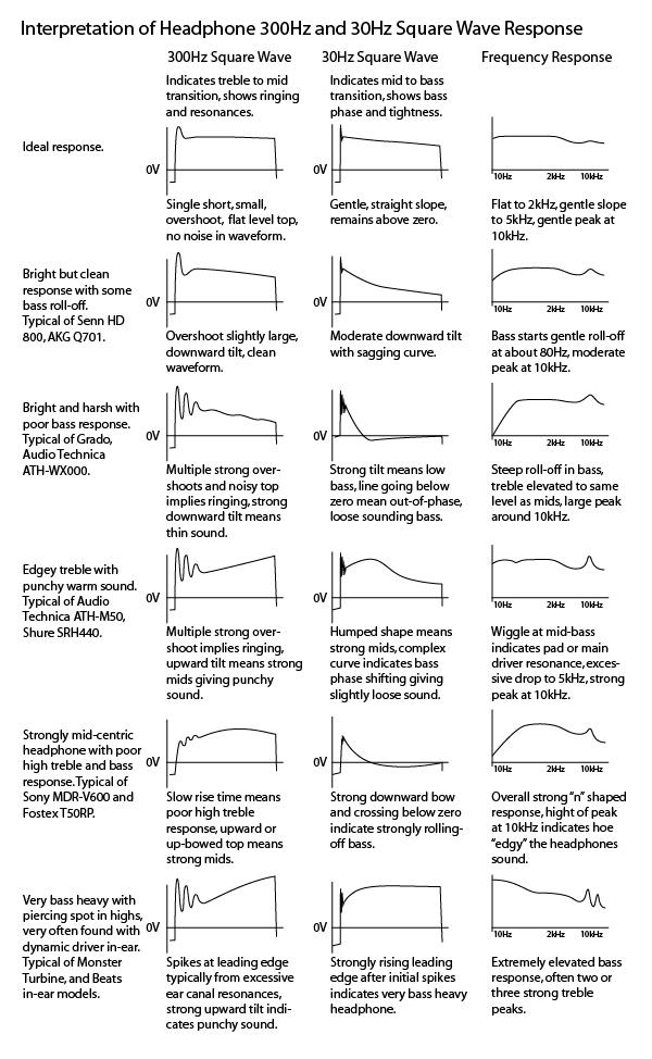
Interpreting Headphone Square Wave Response
The reason why I test square wave response at 300Hz and 30Hz is because the high frequency components of the wave form are tightly squished into the early part of the square wave. So to interpret the treble to mid range we have to "zoom into" the first few moments of the wave form using the 300Hz square wave. When inspecting the mid to bass transition, we have to pull back and look at a longer period of time with the 30Hz square wave. The information from the 300Hz square wave is in the first 10% of the 30Hz wave form, but it's difficult to inspect because it's so compressed.
In the illustration above, you'll find most of the basic information about how to interpret square waves, but I think it's a good idea to look at some actual waveforms and tell you what I see. Generally speaking, I'll be moving from overly bright cans to overly warm ones. Graphs to the left have the 30Hz square wave at the top and the 300Hz square wave below.
Pioneer SE-A1000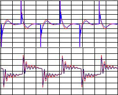 This is a very poorly measuring headphone. From the steeply descending 30Hz square wave we can expect a very bass shy headphone; the significant undershoot below the zero line indicates a sloppy, non-tight bass. The general downward tilt of the 300Hz waveform indicates a thin sound with a stronger treble than mid-range, and very strong first overshoot and strong subsequent ringing make me think these will be very piercing in sound quality. I don't remember listening to these cans...I've probably suppressed the memory of a bad experience. This is a very poorly measuring headphone. From the steeply descending 30Hz square wave we can expect a very bass shy headphone; the significant undershoot below the zero line indicates a sloppy, non-tight bass. The general downward tilt of the 300Hz waveform indicates a thin sound with a stronger treble than mid-range, and very strong first overshoot and strong subsequent ringing make me think these will be very piercing in sound quality. I don't remember listening to these cans...I've probably suppressed the memory of a bad experience.
|
Grado PS1000 From the 30Hz square wave we can see that the low frequency response doesn't extend well into the bass notes, and in going below the zero line indicates some low frequency phase shift that may result in a lack of punch and tightness in the lows. In the 300Hz response we can see an excessive first overshoot and a significant amount of subsequent noise, possibly due to resonances behind the driver in the tubular shaped capsule housing. In listening, I find these headphones bass shy, and very piercing. From the 30Hz square wave we can see that the low frequency response doesn't extend well into the bass notes, and in going below the zero line indicates some low frequency phase shift that may result in a lack of punch and tightness in the lows. In the 300Hz response we can see an excessive first overshoot and a significant amount of subsequent noise, possibly due to resonances behind the driver in the tubular shaped capsule housing. In listening, I find these headphones bass shy, and very piercing.
|
AKG K701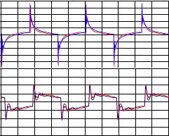 The 30Hz square wave of the K701 presents a fairly strongly descending and bowed waveform, which indicates a fairly strong roll-off in the bass, but it doesn't go below zero, which indicates its bass is tighter than the two headphones above. 300Hz wave shape shows a significantly smaller first overshoot, but one that is still a bit too high for me, likely resulting in the slightly piercing sound of these cans. The remainder of the 300Hz waveform top has little noise showing these cans are nicely damped and will deliver a clear, grain-free sound. The 30Hz square wave of the K701 presents a fairly strongly descending and bowed waveform, which indicates a fairly strong roll-off in the bass, but it doesn't go below zero, which indicates its bass is tighter than the two headphones above. 300Hz wave shape shows a significantly smaller first overshoot, but one that is still a bit too high for me, likely resulting in the slightly piercing sound of these cans. The remainder of the 300Hz waveform top has little noise showing these cans are nicely damped and will deliver a clear, grain-free sound.
|
Sennheiser HD 800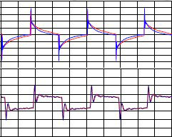 Surprisingly similar to the AKG K701 above, but with somewhat better performance. 30Hz square wave is slightly less bowed downward indicating better bass response. 300Hz plot shows slightly quicker rise time, and slightly less noisy waveform indicating an even more articulate and clean headphone than the K701 above. Waveform is less tilted than the K701 indicating these cans will have a slightly better treble to mid proportion. First overshoot is still too high, however, so the slightly piercing character remains. Surprisingly similar to the AKG K701 above, but with somewhat better performance. 30Hz square wave is slightly less bowed downward indicating better bass response. 300Hz plot shows slightly quicker rise time, and slightly less noisy waveform indicating an even more articulate and clean headphone than the K701 above. Waveform is less tilted than the K701 indicating these cans will have a slightly better treble to mid proportion. First overshoot is still too high, however, so the slightly piercing character remains.
|
Beyerdynamic T70 Here we see in the 30Hz response a headphone with better extended and tighter bass than those so far shown. Waveform top is quite a bit more linear, but small kinks indicate a slightly uneven low to mid response. 300Hz waveform has an overall better shape than the previous two, leading me to believe I'd hear better proportion between treble and mids, and the first overshoot is about the right level. But significant noise and double peak on the leading edge indicate significant resonance, which may make for poorer imaging and a grainy sound. Here we see in the 30Hz response a headphone with better extended and tighter bass than those so far shown. Waveform top is quite a bit more linear, but small kinks indicate a slightly uneven low to mid response. 300Hz waveform has an overall better shape than the previous two, leading me to believe I'd hear better proportion between treble and mids, and the first overshoot is about the right level. But significant noise and double peak on the leading edge indicate significant resonance, which may make for poorer imaging and a grainy sound.
|
Audeze LCD2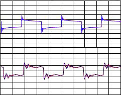 Here we see an essentially perfect 30Hz square wave response with a nearly horizontal and ruler flat waveform top. These cans do indeed have stunning bass response, extremely well extended and tight. The 300Hz wave form has about the right amount of, or maybe slightly low, first overshoot, but it is followed up by a nearly equal in height second spike. I've begun to believe that this second blip is interfering with the ear's ability to discriminate leading edge transients in the audio, which may reduce one's ability to acquire the timing information needed to properly create an audio image. The idea here is that when we see headphones with hash on the front end of the 300Hz square wave, we might be able to predict poor imaging. The remainder of the 300Hz waveform is somewhat non-linear, which may lead to some unevenness in the mid to treble transition, but I've not heard that in particular with these cans. Here we see an essentially perfect 30Hz square wave response with a nearly horizontal and ruler flat waveform top. These cans do indeed have stunning bass response, extremely well extended and tight. The 300Hz wave form has about the right amount of, or maybe slightly low, first overshoot, but it is followed up by a nearly equal in height second spike. I've begun to believe that this second blip is interfering with the ear's ability to discriminate leading edge transients in the audio, which may reduce one's ability to acquire the timing information needed to properly create an audio image. The idea here is that when we see headphones with hash on the front end of the 300Hz square wave, we might be able to predict poor imaging. The remainder of the 300Hz waveform is somewhat non-linear, which may lead to some unevenness in the mid to treble transition, but I've not heard that in particular with these cans.
|
Shure SE535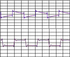 This is one of my favorite in-ear headphones. The 30Hz square wave clearly shows a powerful and linear bass response. The 300Hz square wave shows excellent shape but for one unusual feature: a brief movement in the negative direction prior to moving upward. This is a 3-driver balanced armature headphone with a cross-over circuit. I think what we're seeing here is that the tweeter is out of phase with the other two drivers due to high order filters. Having a driver out of phase relative to other drivers in a multi-way speaker is not uncommon, but I haven't seen it elsewhere with headphones. The rise time of the front of the square wave doesn't look very fast, but you must remember that it's the tweeter going in the negative direction at first that's providing the speed. This is one of those cases where we're not seeing all of the information needed as some phase information is hidden from view. This is one of my favorite in-ear headphones. The 30Hz square wave clearly shows a powerful and linear bass response. The 300Hz square wave shows excellent shape but for one unusual feature: a brief movement in the negative direction prior to moving upward. This is a 3-driver balanced armature headphone with a cross-over circuit. I think what we're seeing here is that the tweeter is out of phase with the other two drivers due to high order filters. Having a driver out of phase relative to other drivers in a multi-way speaker is not uncommon, but I haven't seen it elsewhere with headphones. The rise time of the front of the square wave doesn't look very fast, but you must remember that it's the tweeter going in the negative direction at first that's providing the speed. This is one of those cases where we're not seeing all of the information needed as some phase information is hidden from view.
|
Fostex TH900 Here, we see in the 30Hz square wave a hump early in the wave shape followed by a nice linear trailing down slope. The trailing down slope indicates a tight, well extended bass. The beginning of the hump at the start is magnified in the 300Hz square wave, and indicates stronger mids relative to the highs, and generally leads to a punchy, snappy sound. The first overshoot, however, will deliver a little extra crispness to its reproduction, and the subsequent noise will bring some graininess. Here, we see in the 30Hz square wave a hump early in the wave shape followed by a nice linear trailing down slope. The trailing down slope indicates a tight, well extended bass. The beginning of the hump at the start is magnified in the 300Hz square wave, and indicates stronger mids relative to the highs, and generally leads to a punchy, snappy sound. The first overshoot, however, will deliver a little extra crispness to its reproduction, and the subsequent noise will bring some graininess.
|
Philips L1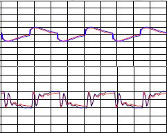 Similar to the Fostex above, the L1's 30Hz square wave indicates a punchy sound and taut, nicely extended bass. This time, however, the leading edge doesn't overshoot, but rather undershoots on the second swing before returning to the waveform top. My experience with this type of headphone is that it has an artificial sounding treble. The only way I can describe it is that it sounds sort of like crinkling the transparent colored cellophane wrapping of fruit baskets. I suspect it will also disturb imaging. Similar to the Fostex above, the L1's 30Hz square wave indicates a punchy sound and taut, nicely extended bass. This time, however, the leading edge doesn't overshoot, but rather undershoots on the second swing before returning to the waveform top. My experience with this type of headphone is that it has an artificial sounding treble. The only way I can describe it is that it sounds sort of like crinkling the transparent colored cellophane wrapping of fruit baskets. I suspect it will also disturb imaging.
|
Koss PortaPro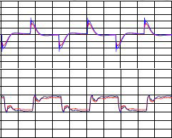 This is an inexpensive and small on-ear headphone that sounds great for what it is. You can see in its 30Hz square wave the bass response is limited, but it doesn't go very far out of phase, so it's tight. The 300Hz square wave doesn't overshoot quite enough, which means its treble transient response is a bit poor, but it doesn't do very much wrong either. Really a stunning result for a compact $40 headphone. This is an inexpensive and small on-ear headphone that sounds great for what it is. You can see in its 30Hz square wave the bass response is limited, but it doesn't go very far out of phase, so it's tight. The 300Hz square wave doesn't overshoot quite enough, which means its treble transient response is a bit poor, but it doesn't do very much wrong either. Really a stunning result for a compact $40 headphone.
|
Sony MDR-V600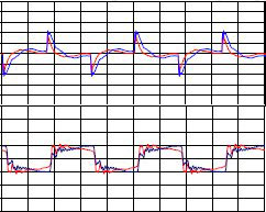 Here's a headphone designed back in the day when mid-heavy headphones that lacked bass and treble responsiveness were pretty much the norm. In fact, I think the V600 is one of the better Sony cans of this type. Here you can see the strongly bowed 30Hz response going somewhat under zero indicating lack of both extension and tightness. And in the 300Hz response a driver struggling to snap up to level. This is a pretty boring headphone. Here's a headphone designed back in the day when mid-heavy headphones that lacked bass and treble responsiveness were pretty much the norm. In fact, I think the V600 is one of the better Sony cans of this type. Here you can see the strongly bowed 30Hz response going somewhat under zero indicating lack of both extension and tightness. And in the 300Hz response a driver struggling to snap up to level. This is a pretty boring headphone.
|
Sony XB500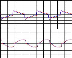 My favorite of the Sony Extra Bass line of headphones, here you can see a headphone that draws a pretty good 30Hz plot with a fairly linear wave top indicating both good extension and bass punch. But the 300Hz leading edge appears to...wait, what leading edge? Yes, treble speed is virtually non-existent with these cans, and the tortuous wriggling the signal does before it finally makes its way to the top about half way through the cycle clearly indicates a great deal of unevenness in the treble to mid transition. In some ways this is not so much a bass-emphasis headphone as a treble/upper-mid reduced one. My favorite of the Sony Extra Bass line of headphones, here you can see a headphone that draws a pretty good 30Hz plot with a fairly linear wave top indicating both good extension and bass punch. But the 300Hz leading edge appears to...wait, what leading edge? Yes, treble speed is virtually non-existent with these cans, and the tortuous wriggling the signal does before it finally makes its way to the top about half way through the cycle clearly indicates a great deal of unevenness in the treble to mid transition. In some ways this is not so much a bass-emphasis headphone as a treble/upper-mid reduced one.
|
Monster Beats Solo HD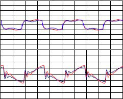 Last, and without doubt among the least, is the Beats by Dre Solo HD. The rounded, broke-back look of its 30Hz square wave is a clear indication of phase problems and indicate a loose, boomy bass. The fact that it remains high in level throughout means you'll have poor quality bass all the way down to 30Hz pummeling your ears. The quick features of the 300Hz leading edge, unlike the XB500 above, means that you'll get a little bit of articulated treble, but the rapidly rising remainder of the waveform indicates it will be overwhelmed by the mids and bass. Last, and without doubt among the least, is the Beats by Dre Solo HD. The rounded, broke-back look of its 30Hz square wave is a clear indication of phase problems and indicate a loose, boomy bass. The fact that it remains high in level throughout means you'll have poor quality bass all the way down to 30Hz pummeling your ears. The quick features of the 300Hz leading edge, unlike the XB500 above, means that you'll get a little bit of articulated treble, but the rapidly rising remainder of the waveform indicates it will be overwhelmed by the mids and bass.
|
Resources
Other articles on headphone measurements on Stereophile, Soundstage, Rin Choi's Blog, and Golden Ears.Udauda's (Rin Choi) Head-Fi Listing of all sites providing headphone measurements, which, unfortunately, doesn't include a link to Marv's measurements at the very bottom of Changstar's home page or the wealth of information in their measurement forum area.
Jude Mansilla (Head-Fi Founder) comments on headphone measurement systems.
- Log in or register to post comments

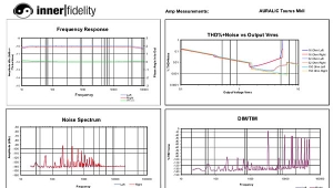
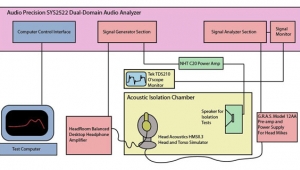


| Loudspeakers Amplification Digital Sources | Analog Sources Accessories Featured | Music Columns Retired Columns | Show Reports | Features Latest News Community | Resources Subscriptions |
 © 2024 Stereophile
AVTech Media Americas Inc., USA
All rights reserved