Digital Processor Reviews

As ALF would say, "There's more than one way to cook a cat." We've been so overwhelmed with linear pulse-code modulation (PCM) recording, we forget there are other ways to pass from the analog domain to the digital.

One of these is delta modulation. The Greek delta (which in its upper-case, block-letter form, looks like an equilateral triangle) is the mathematical symbol for the difference between two quantities; accordingly, in delta modulation, we record not the absolute value of a signal sample, but the difference between successive samples.

Delta modulation isn't new. It's been used for years as a simple way to reduce the necessary bandwidth required to transmit TV signals. Poke your nose up against the CRT, and you'll see that one horizontal line is very much like the preceding or succeeding line. The lines' content doesn't change rapidly, so we don't need much information to describe the difference between one line and the next. If we transmit just the difference information, there's a big reduction in the required bandwidth. (Major changes, which require a lot of transmitted information, are uncommon and don't significantly drive up the bandwidth requirements.)

The same principle can be applied to ordinary PCM. The difference between two samples can never be as large as the absolute maximum level of the program material—sounds do not jump 96dB in 1/50,000th of a second!—so our 16 bits, which would normally cover the full dynamic range of the signal, can be applied to the much narrower range of sample differences. If we designed a system on the assumption that the difference between one sample and the next was never more than 1% of peak signal level (a conservative estimate), we'd gain a 100-fold improvement in resolution! (Not bad.) Or, we could use fewer bits, for resolution comparable to that from conventional PCM. An additional advantage, besides the gain in resolution (or a reduction in bandwidth), is that we no longer have to worry about the signal's absolute level. When we "run out of numbers" in conventional PCM, the signal is clipped to produce a nasty-sounding error. But with a delta-modulation PCM system, the analogous situation produces slew-rate limiting—the recorded difference between samples is not as great as the actual difference—a less offensive distortion.

The problem with such a system, though, is that it requires some pretty hairy hardware. Not only do we have to sample the signal as accurately as in regular PCM, but we have to compute a very accurate difference between successive samples. PCM hardware is complex enough as it is. Why should we have to go to all this trouble for a slight improvement?

There's a way out of this dilemma. Suppose we could make a systematic guess as to what the next sample value would be. By systematic, I mean that the guess is not random. It follows a strict set of rules, so the same set of initial conditions always results in the same guess. Both the encoder and decoder would obey these rules. Therefore, we would only need to transmit the difference between the predicted value of the signal and its actual value. The decoder can figure out the predicted value on its own, then apply the difference signal for correction.

Such a system is called (surprise!) predictive delta modulation. PDM creates an estimated model of the signal in much the same way a painter does a quick sketch on the canvas before he fills in the details, then transmits a code that describes whether the estimate is larger or smaller than the actual value of the next sample. If the sampling is fast enough (greater than about 500kHz), there usually won't be too big a difference between one sample and the next. The difference between the sample and the estimate will then be so small that we can accurately describe it with a code of just one bit!

PDM Explained
The basic PDM circuit (from the dbx manual) is shown in fig.1. It looks complicated, but it's really very simple. There are three sections which I'll explain one at a time.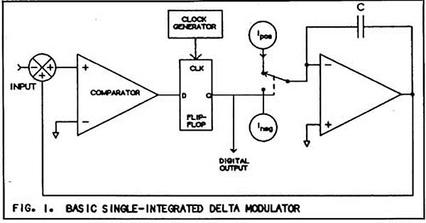

Let's start by saying "Hello!" to our old friend, the capacitor. We can charge a capacitor by applying a voltage to it. The capacitor's charge (in coulombs, footnote 1) is found by multiplying the applied voltage (in volts) by the capacitance (in farads). Or:

Q = CV (I know you've seen that before!)

It works just as well the other way 'round. If we stuff Q amount of charge onto a capacitor, the capacitor's voltage will increase by

V = Q/C

Note that the change in voltage is determined only by the capacitance and the change in charge. A given amount of charge added (or subtracted) will increase (or decrease) the capacitor's voltage by exactly the same amount, regardless of the total amount of charge on the capacitor. Got that? Good.

Now look at the right-hand section of the schematic. The triangle represents a high-gain amplifier. A capacitor is connected from the output to the input. This configuration is called an integrator, because it adds up (integrates) the charge pumped into (or pulled out of) its input.

The exact way the integrator performs its magic is too complicated to go into. (I'd need to explain operational amplifier circuits, an article in itself.) But here's the important part. The injected charge is transferred to the capacitor, and the amplifier's output is the same as the capacitor voltage (given by Q/C). For example, if the capacitor were 2µF, and we pumped in 0.5µC, the output voltage would rise by 0.5/2.0, or 0.25 volts. Likewise, if we pulled out 0.1µC, the voltage would fall by 0.1/2, or 0.05 volts. The integrator is, of course, adding up all these little deposits and withdrawals. Therefore, the instantaneous output of the integrator is simply the running, net charge, divided by the value of the capacitor. Simple, n'est ce pas?

Where does the charge come from? From those two little circles marked Ipos and Ineg. They're charge pumps. One pushes charge, the other pulls. Like the two sides of Alice's mushroom, one makes the total capacitor charge grow larger, the other makes it grow smaller. When either is activated, it inserts (or removes) a precisely defined quantity of charge.

As you should have figured out by now, it's the integrator voltage that models the input signal. By pumping in or pulling out charge, the encoder tries to make the integrator voltage match the input. If the integrator voltage is less than the input, charge is pumped in. If the integrator voltage is greater than the input, charge is removed. But how does the encoder know whether to add or subtract charge?

Easy. It uses a comparator. (That's the triangle on the left.) A comparator is simply a high-gain differential amplifier. That is, it subtracts one input from the other, and amplifies the difference.

Assume the differential amp has a gain of 1 sagan (one billion times). If the difference between its two inputs is 1 billionth of a volt, the output will be 1 volt. Of course, a billionth of a volt is awfully small. (The circuit's random noise is much larger!) 10 microvolts is a more likely difference. 10µV times 1 sagan is 10,000 volts. How do we get 10,000 volts out of an amp that runs on an 18 volt power supply?

We don't. An amplifier's output is limited to the power supply voltage (footnote 2). The amp simply tries its darndest to meet the 10,000V requirement. The result in engineering jargon is that the amp "slams up against the rails." That is, the output jumps up to the power-supply voltage (or down to ground), because that's the highest (lowest) it can go. Which way it jumps depends on the polarity of the difference between the inputs. If it's positive, the amplifier moves to the positive rail, and vice-versa. It's highly unlikely that the integrator's output will ever be close enough to the input to produce a bounded output (ie, one that sits stably between the rails). Therefore, the comparator will constantly jump back and forth, high and low, depending on the relative polarity of the signal input and the comparator output.

Of course, we still haven't explained just how this twitching voltage selects Ipos or Ineg. That's done by the little thingy in the middle. It's called a flip-flop. As you might guess from the name, it's a circuit whose output can take one of two states—high or low. High and low can be any two voltages we like; the important thing is that the flip-flop's output must be one of these two voltages.

There are several types of flip-flops. The one shown here is a D-type ("D" stands for "data"). The flip-flop has a special data input: when the flip-flop is triggered, its output jumps to the same logic level (high or low) as the data input. The trigger signal is simply a steady frequency (in the model 700, it's 644kHz). Each time the trigger goes positive (once per cycle), our D flip-flop is triggered, and the data at the input is transferred to the output. The data, in this case, is the comparator output. Therefore, every time the flip-flop is triggered, its output switches to match the current output state of the comparator.

The little dotted line in the schematic is supposed to suggest that this logic level selects between Ipos and Ineg. Indeed, that's just what happens. The comparator "decides" whether the integrator's output is higher or lower than the signal input. The flip-flop is set to this logic state, which in turn determines whether we will inject or remove charge. And so on, as long as there's an input. (By the way, it's this train of logic highs and lows that constitutes our digitization of the input.) That's it! See how simple it is?

I can already hear objections from The Peanut Gallery. "If all you ever transmit is the difference between the actual and estimated signal values, how can you ever reach the absolute level of the signal? Isn't that what you want to recover?"

Good question. Yes, it's the absolute value we want. Imagine this not-unlikely situation. There's no input. Then—suddenly!—a really big sinewave drops by. The comparator notices that there's like, wow, a really gross difference between the integrator and input voltages. So it doles out one of its little dribs of charge, and 1/644,000th of a second later, compares again. Whoops! It's still behind, so it dumps in some more charge, and so on. Will it ever catch up?

Technically, no. What happens is that the input signal falls behind. The sinewave eventually reaches its peak level, then falls. At some point on its decline, the input voltage drops below the integrator output. At this point, the integrator voltage and the input aren't too different. Everything settles down, with the estimated value close to the absolute value.

---

Footnote 1: A coulomb is an Avogadro's number's-worth of electrons, about 6E²³. It's named after Melvin Coulomb, the French music-hall comic who discovered how easy it was to build up an enormous static charge by shuffling across the carpet. Mel died tragically, the victim of a jealous husband whose wife's derriere he (Mel) had zapped once too often. In accordance with French legal precedent, the husband was acquitted.

Footnote 2: We assume there's no output transformer to step it up.