Sidebar 3: Measurements
For logistical reasons, I measured a different sample of the Magico S2 from those auditioned by RvB. Mine had the serial number 25106. I used DRA Labs' MLSSA system and a calibrated DPA 4006 microphone with an Earthworks microphone preamplifier to measure the Magico S2's farfield frequency behavior and dispersion with the 132lb loudspeaker raised off the floor on a dolly. I took a full set of farfield measurements with the microphone at my usual 50" distance on the tweeter axis, then repeated the measurements with the microphone 1m away to check that aggressively windowing the MLSSA time-domain data at the further distance, to eliminate the floor bounce of the woofer outputs, wasn't reducing the measured behavior's midrange resolution. (It didn't.) I used an Earthworks QTC-40 mike, which has a small, ¼"-diameter capsule, for the nearfield responses.
Footnote 1: EPDR is the resistive load that gives rise to the same peak dissipation in an amplifier's output devices as the loudspeaker. See "Audio Power Amplifiers for Loudspeaker Loads," JAES, Vol.42 No.9, September 1994, and stereophile.com/reference/707heavy/index.htm. Footnote 2: This means that the loudspeaker is firing into hemispherical space rather than a full sphere. A speaker that has a truly flat response in the usual "4pi" space will therefore appear to have a boosted upper-bass output with a nearfield measurement, the center frequency of that boost depending on the physical dimensions of the speaker and the woofer alignment. See this explanation or aes2.org/publications/elibrary-page/?id=7171.
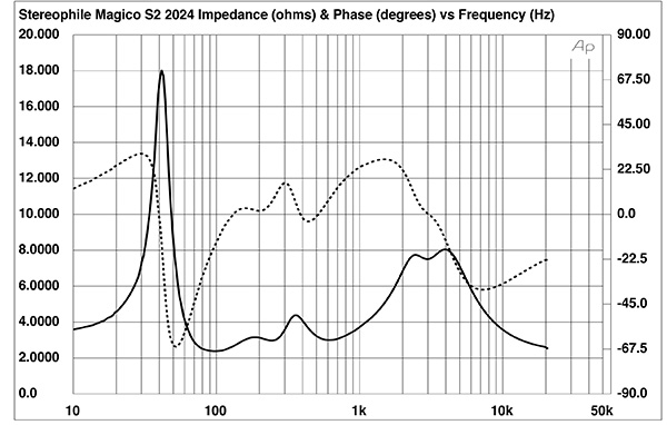
Fig.1 Magico S2, electrical impedance (solid) and phase (dashed) (2 ohms/vertical div.).
Magico specifies the S2's sensitivity as 86.5dB. My B-weighted estimate was slightly higher, at 87.5dB(B)/2.83V/1m. The S2's impedance is specified as 4 ohms. My measurement, made with Dayton Audio's DATS V2 system (fig.1, solid trace), dropped below 4 ohms between 60Hz and 322Hz, between 405Hz and 1100Hz, and above 8.5kHz. The minimum values were 2.4 ohms between 85Hz and 110Hz, and 3 ohms between 590Hz and 725Hz. The electrical phase angle (dashed trace) is often high; as a result, the effective resistance, or EPDR (footnote 1), drops below 3 ohms between 10Hz and 33Hz and between 47Hz and 380Hz, and below 2 ohms between 51Hz and 118Hz and in several other regions between 263Hz and 20kHz. The minimum EPDR values are 0.94 ohm at 69Hz, 1.74 ohms at 912Hz, and 1.25 ohms at 15.5kHz. As music can have high levels at the two lower frequencies, the S2 will demand a lot of current from the partnering amplifier.
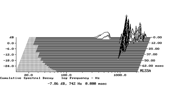
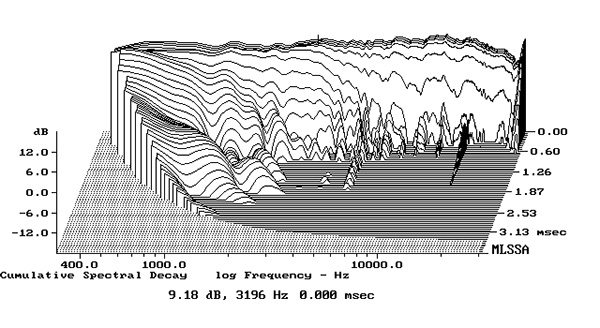
Fig.2 Magico S2, cumulative spectral decay plot calculated from the output of an accelerometer fastened to the rear of the curved sidewall level with the lower woofer (MLS driving voltage to speaker, 7.55V; measurement bandwidth, 2kHz.).
The enclosure seemed inert, though when I rapped the surfaces with my knuckles I heard faint "plinks," suggesting that any resonances were usefully high in frequency. The loudest "plinks" were on a vertical section of the curved rear panel. Using a plastic-tape accelerometer, I found some resonant modes between 740Hz and 1kHz in this area (fig.2). As well as having high frequencies, these modes have a high Q (Quality Factor); these modes are unlikely to have audible consequences.
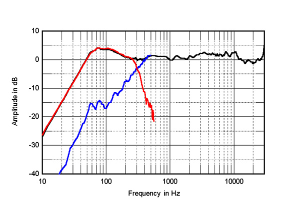
Fig.3 Magico S2, anechoic response on tweeter axis at 50", averaged across a 30° horizontal window and corrected for microphone response, with the nearfield responses of the woofers (red), midrange unit (blue), and their complex sum (black), respectively plotted below 550Hz, 500Hz, and 310Hz.
The peak at 42Hz in the impedance magnitude trace in fig.1 suggests that this is the tuning frequency of the woofers' sealed-box loading. The red trace in fig.3 shows the summed nearfield response of the two woofers, which behaved identically. The 4dB rise in the midbass region is due to the nearfield measurement technique, which assumes that the drive units are mounted in a true infinite baffle (footnote 2). As expected, the woofers' output is down by 6dB at the tuning frequency, which is the lowest note on the double bass and four-string electric bass guitar. The woofers cross over to the midrange unit (fig.3, blue trace, plotted in the ratio of the square root of its radiating area to that of the woofers) at 300Hz. (The discontinuity between 55Hz and 90Hz in the midrange unit's high-pass rolloff in this graph is due to crosstalk from the woofers. As there is only a single pair of binding posts, it wasn't possible to measure the midrange unit's and woofers' nearfield responses in isolation from each other.)
The black trace above 310Hz in fig.3 shows the S2's quasi-anechoic farfield response, averaged across a 30° horizontal window centered on the tweeter axis. There is a very slight lack of energy at the top of the midrange unit's passband, but the response is otherwise smooth and even, falling within tight ±1dB limits. The output slopes gently down by 3dB in the top octave before starting to rise at 20kHz. It peaks between 30kHz and 40kHz (not shown in this graph) due to the tweeter's fundamental dome resonance.
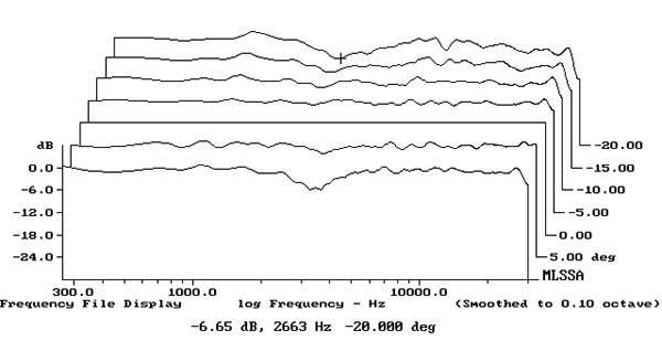
Fig.4 Magico S2, lateral response family at 50", normalized to response on tweeter axis, from back to front: differences in response 90–5° off axis, reference response, differences in response 5–90° off axis.
Fig.5 Magico S2, vertical response family at 50", normalized to response on tweeter axis, from back to front: differences in response 20–5° above axis, reference response, differences in response 5–10° below axis.
Fig.4 shows the S2's horizontal dispersion, normalized to the response on the tweeter axis, which thus appears as a straight line. While the dispersion narrows in the top two octaves, the radiation pattern is impressively even, which correlates with accurate and stable stereo imaging. The speaker's radiation pattern in the vertical plane, again normalized to the response on the tweeter axis, which is 38" from the floor with the speaker supported on its feet, is shown in fig.5. The loud speaker's response doesn't change appreciably 5° above or below the tweeter axis, which is appropriate for seated listeners. A suckout at 2.7kHz develops more than 15° above and 5° below the tweeter axis, suggesting that this is the crossover frequency between the midrange unit and tweeter.
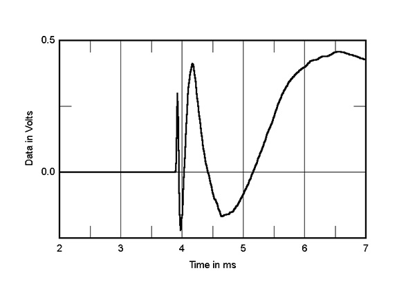
Fig.6 Magico S2, step response on tweeter axis at 50" (5ms time window, 30kHz bandwidth).
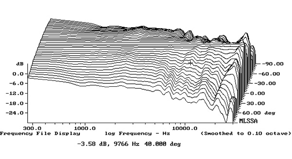
Fig.7 Magico S2, cumulative spectral-decay plot on tweeter axis at 50" (0.15ms risetime).
In the time domain, the Magico S2's step response (fig.6) indicates that all four drive units are connected in positive acoustic polarity. The tweeter's output arrives first at the microphone, followed first by that of the midrange unit, then by that of the woofers. The decay of each drive unit's step smoothly blends with the start of the step of the unit next lower in frequency, which implies optimal crossover implementation. The S2's cumulative spectral decay, or waterfall, plot (fig.7) is very clean overall. (As always with my cumulative spectral decay plots, ignore the ridge of delayed energy close to 16kHz, which is due to interference from the MLSSA host PC's video circuitry.)
The Magico S2 offers excellent measured performance.—John Atkinson
Footnote 1: EPDR is the resistive load that gives rise to the same peak dissipation in an amplifier's output devices as the loudspeaker. See "Audio Power Amplifiers for Loudspeaker Loads," JAES, Vol.42 No.9, September 1994, and stereophile.com/reference/707heavy/index.htm. Footnote 2: This means that the loudspeaker is firing into hemispherical space rather than a full sphere. A speaker that has a truly flat response in the usual "4pi" space will therefore appear to have a boosted upper-bass output with a nearfield measurement, the center frequency of that boost depending on the physical dimensions of the speaker and the woofer alignment. See this explanation or aes2.org/publications/elibrary-page/?id=7171.