Sidebar 2: Measurements
The DQ-12s did very well on the LEDR test from the Chesky Test CD. LEDR is short for "Listening Environment Diagnostic Recording" and is described in detail in Vol.12 No.12. In short, it reveals a speaker's (and the room's) ability to present images in their correct spatial location. (I highly recommend this recording for evaluating speakers and listening rooms.) After my favorable impression of the DQ-12s' imaging and soundstage presentation, I was not surprised that they performed well on the LEDR test, throwing a solid image between and above the speakers.
Driving the DQ-12 with a sinewave oscillator revealed fairly strong cabinet resonances at 275, 220, and 195, with excess output also noted at 60 and 40Hz. The 195Hz mode was the most severe, causing a rattling sound to emanate from the rear of the enclosure.
Fig.1 shows how the DQ-12's impedance magnitude and phase vary with frequency. The woofer peak at 45Hz can be seen, perhaps equating with the excessive 40Hz output. The impedance never drops below 4 ohms, implying that it will be a fairly easy load to drive with most amplifiers.
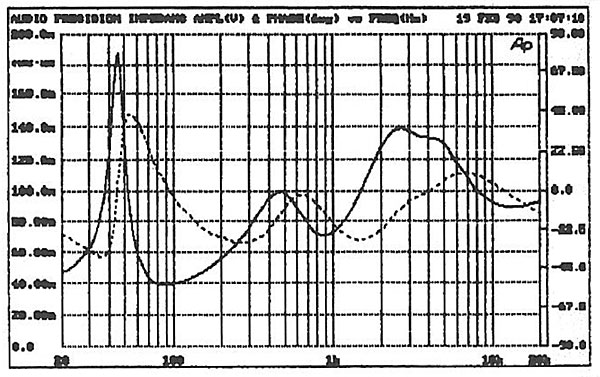
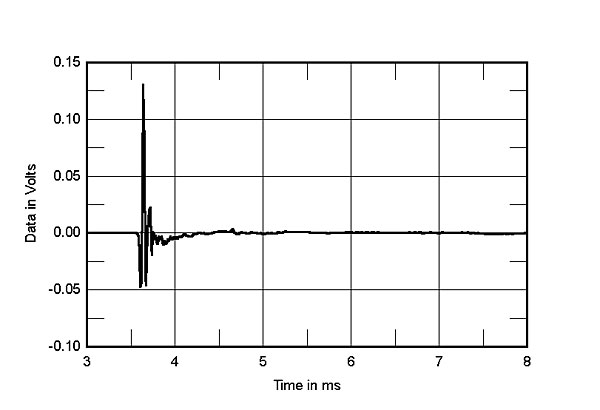
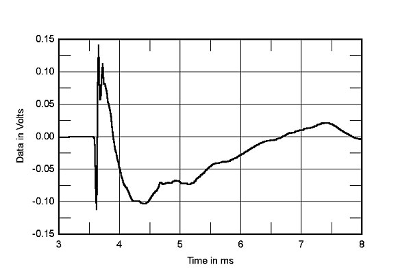
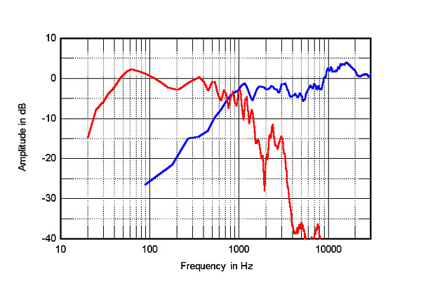
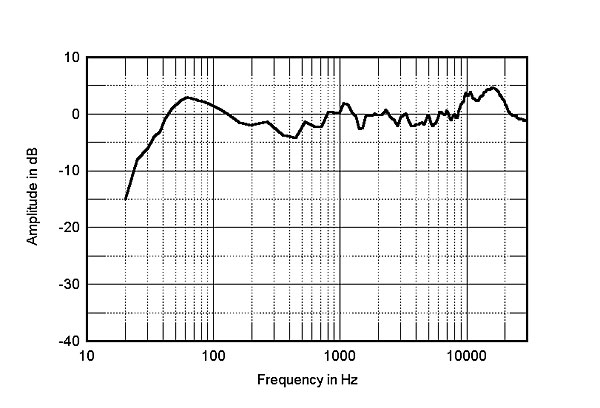
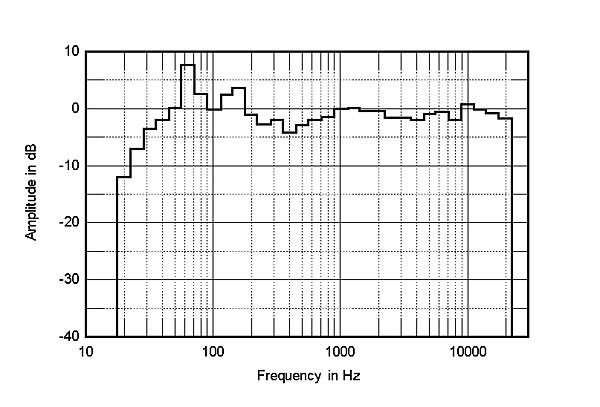
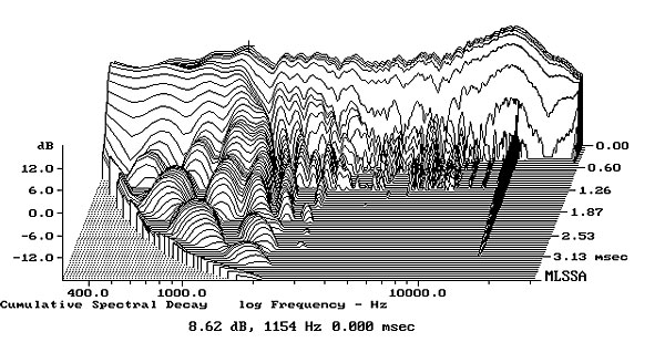
Fig.1 Dahlquist DQ-12, impedance magnitude (solid trace) and electrical phase (dotted) (5 ohms/vertical div.; note that the measured phase angle is inverted.
Looking at the DQ-12's MLSSA-derived impulse response 48" away on the tweeter axis (fig.2) reveals a reasonably time-coherent signal with the tweeter apparently connected in the opposite polarity to that of the woofer and midrange. Fig.3 shows the step response.
Fig.2 Dahlquist DQ-12, impulse response on HF axis at 48" (5ms time window).
Fig.3 Dahlquist DQ-12, step response on HF axis at 48" (5ms time window).
Windowing the anechoic portion of the impulse response to remove room reflections and performing an FFT calculation gives the speaker's anechoic response. The DQ12's biwiring capability makes it easy to look at the woofer and midrange/tweeter responses separately, both shown in fig.4. (The level matching of the two curves in fig.4 is only approximate.) Several woofer cone-breakup modes are clearly visible, starting just above the crossover point (400Hz). Given the DQ-12's gentle crossover slope, the modes below 3kHz may not be sufficiently attenuated to be inaudible and will add a sense of liveliness if not quite brightness to the sound. A peak in the midrange unit's response is also apparent at 1kHz, though the overall midrange trend is smooth. The most prominent feature, however, is the excess of high-frequency energy, starting at 5kHz but really taking off above 8kHz. This will correspond to my subjective impression of the speaker having a bright, forward treble balance overall.
Fig.4 Dahlquist DQ-12, acoustic crossover on HF axis at 48" with nearfield woofer response.
The problem with FFT-derived frequency responses is that they tend to reveal almost too much detail in the treble. To look at the speaker's full-range response, therefore, I took several impulse responses across a 30° arc at the same 48" microphone distance and averaged the resultant responses, this removing the contribution of small interference effects. The result is shown to the right of fig.5, married to the woofer's response measured in the nearfield; ie, with the microphone almost touching the dustcap. The bass appears to be rather underdamped, as suggested by the auditioning. The midband is relatively flat, with a few small peaks in the presence region that may contribute to a brightish impression. Again, the severe increase in energy above 8kHz is apparent, despite this curve incorporating the output of the speaker up to 15° off-axis laterally.
Fig.5 Dahlquist DQ-12, response averaged across 30° horizontal window centered on HF axis with nearfield woofer response.
The spatially averaged, in-room response, assessed on a third-octave basis (fig.6), is what I would have predicted from the auditioning: peaky treble, smooth midband, and somewhat lumpy mid/upper bass. It should be noted that spatially averaging the response effectively removes the effect of room resonances from the measurement. Also apparent is a slight lack of energy around the woofer/midrange crossover region. The fact that this plot was made with a completely different microphone and measuring system (AudioControl Industrial SA-3050A) confirms that the HF response rise is real.
Fig.6 Dahlquist DQ-12, 1/3-octave, spatially averaged response in RH listening room.
Fig.7 shows the MLSSA-derived cumulative spectral-decay plot, also referred to as a "waterfall" graph. A few strong resonances centered around 1kHz are apparent as "ridges" running parallel to the time axis, although the upper midrange and treble decay is quite clean. The peak in the top octave appears to be more of an equalization or diffraction-related effect than a resonance, although it just might have a very low Q. (The sharp line about 16kHz is not part of the speaker response, but rather the 15,750Hz scanning frequency of the computer monitor used.) Looking at only the woofer's cumulative spectral decay (not shown), a significant resonant ridge was apparent in the lower midrange, probably due to a cabinet resonance problem.—Robert Harley
Fig.7 Dahlquist DQ-12, cumulative spectral decay plot on HF axis at 48".