
It must be noted, of course, that the error voltage induced by the changing external field dominates, so this result would be largely masked. (The greater the conductor spacing, the greater the masking.) With loudspeaker cables (greater than, say, 2mm in diameter) that are terminated close to their characteristic impedance, the external fields will contribute minimal error. However, the loss field still produces time dispersion. If the error voltage is to be correctly predicted, skin depth must be included, a simple resistive model being inaccurate. I am not trying to say that this effect is necessarily significant, only that an error component is predicted by our theory and is shown by the measurements to exist.
Multiple conductors
At this juncture, it is interesting—may I be so bold as to say fun?—to conjecture both what happens to an electromagnetic loss field propagating through a copper conductor when it encounters an abrupt discontinuity in conductivity, and whether this has any correlation with defects in copper that are attributable to crystal boundary interfaces. Consider a long transmission line terminated in its characteristic impedance. Electromagnetic energy entering the line will propagate in a uniform manner, finally being absorbed in the load (just as with a VHF aerial cable which is terminated in 75 ohms). However, if the termination is in error, then a proportion of the incident energy is reflected back along the cable toward the source. In extreme cases, where there is either an open or a short-circuit load, then all the incident energy is reflected, though for a short circuit the sign of the E-Bar field is reversed upon reflection, thus canceling the electric field in the cable and informing the source that there is a short-circuit termination.
The point to observe is that a discontinuity in the characteristic impedance results in at least partial reflection at the discontinuity, which will distort the time-domain waveform. This reflective property of a change in characteristic impedance is used to locate faults in long lengths of cable by using time-domain reflectometry—a pulse is transmitted along the cable, and the return times of the partial echoes from each discontinuity indicate the location of the fault.
Similarly, for a wave traveling in copper, an impedance discontinuity (read here micro-discontinuity) leads to partial reflection centered on the discontinuity. This effect must be compounded with an already dispersive propagation—ie, different frequencies propagate at different velocities—thus time-smearing the error signal or loss wave in the conductor.
Now let's play to the gallery...This observation gives insight into the possible effects of crystal boundaries within copper, where each boundary can be viewed as a discontinuity in conductivity and corresponds to zones of localized partial reflection for the radial loss field.
Note, however, that this property is not necessarily nonlinear. We do not have to invoke a semiconductor-type non-linearity to identify a problem; we're probably talking here of mainly linear errors. So we would not necessarily expect to observe either a significant reading on the distortion-factor meter, or modulation noise or sidebands in high-resolution spectral analysis, for steady-state excitation. However, just as with loudspeaker measurements (which often show non–minimum-phase behaviour), amplitude-only response measurements do not give a complete representation of stored energy and time-delay mechanisms. We would require very careful measurements directly of the errors for both amplitude and phase, or of impulse response in the time domain.
Following the comments on the error function in an earlier "Essex Echo" article (footnote 3), direct measurements of the output signal will in general yield insufficient accuracy to allow a true estimate of the system error. This point is worth thinking about: Ideally, we need to assess the actual current distribution in the conductors; or, more realistically, to measure the conductor error directly.
Real-life boundaries
The final stage in the development of our model is to account for copper conductors of finite thickness, where the thickness may well be much less than the skin depth. Just as a wave traveling in air is reflected when confronted by a short-circuit, so a wave that encounters an open circuit (eg, a copper/air boundary) while traveling in a conductor also undergoes reflection and therefore passes back into the conductor, undergoing further attenuation as it does so. However, the boundary conditions require a reversal of the magnetic field. Provided the thickness of the conductor is much less than the skin depth, therefore, the incident and reflected H-Bar fields nearly cancel, and the conductor exhibits a lower internal magnetic field. Consequently there is predominantly an axial electric field and corresponding axial conduction current, the conductor behaves nearly as a pure resistor, and the magnetic field—hence the inductive component—is reduced to the pseudo-static case. The current distribution is nearly uniform. The conductor has lost its memory.
Impedances
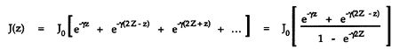
Because we are dealing with a propagation phenomenon, the traveling-wave model can be used to evaluate the component of conductor impedance due to the internal fields. Since non-Litz conductor radii range at most to a few millimeters, the internal wave will undergo reflection at the conductor boundary due to the gross impedance mismatch between dielectric and conductor. I must own up that this area of the analysis is more difficult; at best, the results are approximate due to the cylindrical geometry. Consequently, when you write your letters of complaint, please address them directly to John Atkinson! A contrived rectangular conductor geometry is shown in fig.8. Let the current density be J0 at boundary A, where the loss wave propagates in the z direction; note that the current is aligned with the elemental conductor length ΔL. As the wave propagates from boundary A toward boundary B, it undergoes attenuation as the conductor has high conductivity. At boundary B there is total reflection due to the impedance mismatch. Similarly, the returned wave is re-reflected at A, and so on at subsequent boundary encounters. Considering these multiple-boundary reflections and noting the attenuation and phase over a length z is e–γz, Fig.8 "Contrived" conductor geometry for skin-depth calculation.
 The total current I is calculated by integrating J(z) over the conductor cross-section,
 For a good conductor, α = β = 1/δ and γ = α + jβ = (1 + j)/δ, whereby
J0 = I(1+j)/(Wδ)
The voltage ΔV appearing across an axial length of conductor ΔL is calculated from the surface electric field E; however, noting J = σE, then ΔV = E ΔL = J(z=0) ΔL/σ and substituting from the hyperbolic family of functions,
For a good conductor, α = β = 1/δ and γ = α + jβ = (1 + j)/δ, whereby
J0 = I(1+j)/(Wδ)
The voltage ΔV appearing across an axial length of conductor ΔL is calculated from the surface electric field E; however, noting J = σE, then ΔV = E ΔL = J(z=0) ΔL/σ and substituting from the hyperbolic family of functions,
 Although contrived, the final result demonstrates a reasonable approximation of the internal impedance, assuming a nongranular conductivity. As a final step, transform the expression for Zint(Z), noting
 and Rint = Zint(Z) at zero frequency; ie, the DC resistance/meter, Rint(Z) = (WZσ)–1
 This final expression allows an independent selection of conductor DC resistance and conductor radius (in a multistrand construction), assuming the skin depth δ is known (δ is a function of ω, µ, and σ).
Although there is a limit on the maximum conductor radius for a given DC resistance/meter and material conductivity, for a cylindrical conductor of radius Z which is equal to or less than √(Π σ Rint), a Litz cable may be assembled from a number of paralleled and individually insulated conductors. With such a construction, the transition frequency at which skin depth becomes significant can be controlled. At low frequencies, where δ is greater than Z, the internal impedance of a conductor is substantially resistive. For δ smaller than Z—the wire is greater in diameter than the skin depth—the internal impedance is proportional to the square root of the frequency, with a phase shift approaching 45°.
The critical frequency, fc, follows approximately from the expression for α (α = 1/δ = 1/Z) where fc = 1/(ΠµσZ2). For a cable with a diameter of 0.8mm, therefore, fc = 27kHz. (This result is approximate, as the cylindrical geometry has not been fully accounted for in the analysis. [Maybe it might turn out that a cylindrical conductor is less optimal than a rectangular, something that has been postulated by both Madrigal and TARA Labs.—Ed.]) We therefore conclude that, for the internal impedance taken over the audio band, a thin conductor behaves as a resistor, whereas a thick conductor has a complex (frequency-dependent) impedance.
In this latter discussion we have interpreted our model in the steady-state and as a lumped impedance. However, we should not lose sight of the time-domain model and the extension to a discontinuous or granular conductivity. As observed in the earlier "Echo" article (footnote 4), steady-state analysis, though correct, can limit our appreciation of a system. We would not expect to observe all anomalies easily on steady-state tests. As they can be hidden from view when the errors are of low level, such tests can be insensitive. Alternatively, direct measures of errors should be sought rather than attempting to extract them from a dominant signal.
In developing this model we have concentrated on the loss mechanism inherent in the conductors. We have not discussed the characteristic impedance observed at the input of the interconnect. This is a direct result of the amount of energy stored in the electric and magnetic fields needed to "fill" the cable—ie, the propagating energy within the cable system.
Ultimately, the energy loss in the interconnect is a function of the characteristic impedance, the cable length, and the load termination, as these directly influence the loss field, hence the conductor current, hence the voltage across the cable length. The load impedance that terminates the line is mapped into the interconnect error mechanisms. This latter observation is very important with loudspeaker loads, many of which are nonlinear. Much of the error attributable to loudspeaker cable is a consequence of the nonlinear load impedance acting with the series impedance of the cable—this must include the effect of skin depth.
This final expression allows an independent selection of conductor DC resistance and conductor radius (in a multistrand construction), assuming the skin depth δ is known (δ is a function of ω, µ, and σ).
Although there is a limit on the maximum conductor radius for a given DC resistance/meter and material conductivity, for a cylindrical conductor of radius Z which is equal to or less than √(Π σ Rint), a Litz cable may be assembled from a number of paralleled and individually insulated conductors. With such a construction, the transition frequency at which skin depth becomes significant can be controlled. At low frequencies, where δ is greater than Z, the internal impedance of a conductor is substantially resistive. For δ smaller than Z—the wire is greater in diameter than the skin depth—the internal impedance is proportional to the square root of the frequency, with a phase shift approaching 45°.
The critical frequency, fc, follows approximately from the expression for α (α = 1/δ = 1/Z) where fc = 1/(ΠµσZ2). For a cable with a diameter of 0.8mm, therefore, fc = 27kHz. (This result is approximate, as the cylindrical geometry has not been fully accounted for in the analysis. [Maybe it might turn out that a cylindrical conductor is less optimal than a rectangular, something that has been postulated by both Madrigal and TARA Labs.—Ed.]) We therefore conclude that, for the internal impedance taken over the audio band, a thin conductor behaves as a resistor, whereas a thick conductor has a complex (frequency-dependent) impedance.
In this latter discussion we have interpreted our model in the steady-state and as a lumped impedance. However, we should not lose sight of the time-domain model and the extension to a discontinuous or granular conductivity. As observed in the earlier "Echo" article (footnote 4), steady-state analysis, though correct, can limit our appreciation of a system. We would not expect to observe all anomalies easily on steady-state tests. As they can be hidden from view when the errors are of low level, such tests can be insensitive. Alternatively, direct measures of errors should be sought rather than attempting to extract them from a dominant signal.
In developing this model we have concentrated on the loss mechanism inherent in the conductors. We have not discussed the characteristic impedance observed at the input of the interconnect. This is a direct result of the amount of energy stored in the electric and magnetic fields needed to "fill" the cable—ie, the propagating energy within the cable system.
Ultimately, the energy loss in the interconnect is a function of the characteristic impedance, the cable length, and the load termination, as these directly influence the loss field, hence the conductor current, hence the voltage across the cable length. The load impedance that terminates the line is mapped into the interconnect error mechanisms. This latter observation is very important with loudspeaker loads, many of which are nonlinear. Much of the error attributable to loudspeaker cable is a consequence of the nonlinear load impedance acting with the series impedance of the cable—this must include the effect of skin depth.
Footnote 3: Malcolm Omar Hawksford, "The Essex Echo: on errors, low feedback and fuzzy distortion," HFN/RR, September 1984, Vol.29 No.9, pp.37–41. Footnote 4: Hawksford, ibid.
At this juncture, it is interesting—may I be so bold as to say fun?—to conjecture both what happens to an electromagnetic loss field propagating through a copper conductor when it encounters an abrupt discontinuity in conductivity, and whether this has any correlation with defects in copper that are attributable to crystal boundary interfaces. Consider a long transmission line terminated in its characteristic impedance. Electromagnetic energy entering the line will propagate in a uniform manner, finally being absorbed in the load (just as with a VHF aerial cable which is terminated in 75 ohms). However, if the termination is in error, then a proportion of the incident energy is reflected back along the cable toward the source. In extreme cases, where there is either an open or a short-circuit load, then all the incident energy is reflected, though for a short circuit the sign of the E-Bar field is reversed upon reflection, thus canceling the electric field in the cable and informing the source that there is a short-circuit termination.
The final stage in the development of our model is to account for copper conductors of finite thickness, where the thickness may well be much less than the skin depth. Just as a wave traveling in air is reflected when confronted by a short-circuit, so a wave that encounters an open circuit (eg, a copper/air boundary) while traveling in a conductor also undergoes reflection and therefore passes back into the conductor, undergoing further attenuation as it does so. However, the boundary conditions require a reversal of the magnetic field. Provided the thickness of the conductor is much less than the skin depth, therefore, the incident and reflected H-Bar fields nearly cancel, and the conductor exhibits a lower internal magnetic field. Consequently there is predominantly an axial electric field and corresponding axial conduction current, the conductor behaves nearly as a pure resistor, and the magnetic field—hence the inductive component—is reduced to the pseudo-static case. The current distribution is nearly uniform. The conductor has lost its memory.
Because we are dealing with a propagation phenomenon, the traveling-wave model can be used to evaluate the component of conductor impedance due to the internal fields. Since non-Litz conductor radii range at most to a few millimeters, the internal wave will undergo reflection at the conductor boundary due to the gross impedance mismatch between dielectric and conductor. I must own up that this area of the analysis is more difficult; at best, the results are approximate due to the cylindrical geometry. Consequently, when you write your letters of complaint, please address them directly to John Atkinson! A contrived rectangular conductor geometry is shown in fig.8. Let the current density be J0 at boundary A, where the loss wave propagates in the z direction; note that the current is aligned with the elemental conductor length ΔL. As the wave propagates from boundary A toward boundary B, it undergoes attenuation as the conductor has high conductivity. At boundary B there is total reflection due to the impedance mismatch. Similarly, the returned wave is re-reflected at A, and so on at subsequent boundary encounters. Considering these multiple-boundary reflections and noting the attenuation and phase over a length z is e–γz,
Fig.8 "Contrived" conductor geometry for skin-depth calculation.
The total current I is calculated by integrating J(z) over the conductor cross-section,
For a good conductor, α = β = 1/δ and γ = α + jβ = (1 + j)/δ, whereby
J0 = I(1+j)/(Wδ)
The voltage ΔV appearing across an axial length of conductor ΔL is calculated from the surface electric field E; however, noting J = σE, then ΔV = E ΔL = J(z=0) ΔL/σ and substituting from the hyperbolic family of functions,
Although contrived, the final result demonstrates a reasonable approximation of the internal impedance, assuming a nongranular conductivity. As a final step, transform the expression for Zint(Z), noting
and Rint = Zint(Z) at zero frequency; ie, the DC resistance/meter, Rint(Z) = (WZσ)–1
This final expression allows an independent selection of conductor DC resistance and conductor radius (in a multistrand construction), assuming the skin depth δ is known (δ is a function of ω, µ, and σ).
Although there is a limit on the maximum conductor radius for a given DC resistance/meter and material conductivity, for a cylindrical conductor of radius Z which is equal to or less than √(Π σ Rint), a Litz cable may be assembled from a number of paralleled and individually insulated conductors. With such a construction, the transition frequency at which skin depth becomes significant can be controlled. At low frequencies, where δ is greater than Z, the internal impedance of a conductor is substantially resistive. For δ smaller than Z—the wire is greater in diameter than the skin depth—the internal impedance is proportional to the square root of the frequency, with a phase shift approaching 45°.
Footnote 3: Malcolm Omar Hawksford, "The Essex Echo: on errors, low feedback and fuzzy distortion," HFN/RR, September 1984, Vol.29 No.9, pp.37–41. Footnote 4: Hawksford, ibid.


