As shown in fig.1, a propagating electromagnetic wave consists of an oscillation of energy between the magnetic and electric fields, these akin to kinetic and potential energy in a mechanical system. It is helpful to think of free-space dielectrics and conductors as distributed inductance-capacitance-resistance networks. For example, in a coaxial cable (fig.3), the electric field is everywhere radial, while the magnetic field forms concentric circles around the inner conductor (Ampere's Circuital Law). It is important to note, as commented upon earlier, that the E-Bar and H-Bar fields are both spatially at right angles to each other and to the direction of propagation, which is along the axis of the cable. This is a direct result of Maxwell's Equations.
 Fig.3 Cross-section of coaxial cable showing radial E-Bar field and circumferential H-Bar field.
Power flow
Fig.3 Cross-section of coaxial cable showing radial E-Bar field and circumferential H-Bar field.
Power flow
In an electromagnetic system, the "power flow" is a directed or vector quantity and is represented as a power-density function P-Bar (watt/m2) called the Poynting Vector, where P-Bar = E-Bar x H-Bar (with x being the vector crossproduct rather than the conventional multiplication symbol). For a coaxial cable, P-Bar is directed axially, indicating that energy is propagated along the cable. Integrate P-Bar over a cross-section of area (between the conductors) and the result is the total power carried by the cable. The expression for P-Bar can be compared with power calculations in lumped electrical systems, where P (power) = V (voltage) x I (current) (ie, V is equivalent to the E-Bar field, I to the H-Bar field).
If we assume that the two conductors of the coaxial cable are ideal (where σ approaches infinity), then all the electromagnetic energy flows through the dielectric (insulator) because the electric field within the conductors must be zero. The E-Bar field does not penetrate the conductors, the skin depth is zero (check back to the expression for δ), and the conductors act as perfect reflectors (that's why a mirror is coated with a good conductor). In this ideal case, there is only a surface current on each conductor to match the boundary condition for the tangential magnetic field H-Bar at the dielectric/conductor interface (see Skilling [2]). You should visualize a wave traveling in an axial direction within the dielectric and being guided by the conductors, where the electric and magnetic fields are both at right angles to each other and to the direction of propagation along the axis of the cable.
However, this perfect example is unrealistic. All practical conducting materials have a finite conductivity σ. They must inevitably exhibit an energy loss because, at the molecular level, collisions convert electrical energy into heat.
As the wave propagates through the dielectric, a study of the boundary condition reveals that the radial electric field E-Bar is not quite at 90° to the conductor surface. This is a direct consequence of the finite conductivity producing a longitudinal component, E-Barσ, which is the voltage drop (in V/m) along the wire. The wave no longer takes the shortest path through the dielectric surrounding the conductor, but appears to travel more slowly at the conductor surface (rather in the way flowing water close to a river bank gives a curved velocity profile).
At each dielectric-to-conductor interface, a refracted field results within the conductor (the longitudinal E-Barσ field) which proceeds to propagate radially at virtual right angles to the axis of the cable into the interior of the conductor. This field we shall call the "loss field." Consequently, the majority of the electromagnetic energy propagates in a near-axial direction within the dielectric, but a much-reduced loss field propagates almost radially into each conductor.
The electric field Eσ is oriented axially along the length of the conductor while the H field remains circumferential, curling around the internal longitudinal current. The Poynting Vector of the loss field is therefore directed radially into the conductor. It is the propagation of this loss field in a radial direction that is controlled by the material parameters of the conductors (µ, σ, ε) and is ultimately attenuated by conversion to heat. It is here that the story becomes more relevant to audio.
To summarize, real-world conductors have finite conductivity, which causes the guided electromagnetic energy traveling in the dielectric between the conductors to spill out and propagate into the interior of each conductor. Although the main component of energy propagates rapidly within the dielectric along the axis of the cable, the energy constituting the loss field that enters the conductor across the boundary propagates much more slowly (see Table 2), being determined by the frequency-dependent parameters α and β. In a perfect conductor, a current traveling only in the surface would match the boundary conditions for the axial propagating field. (Maybe you recall from Gauss's Theorem that the lines of the displacement vector D-Bar must terminate on a surface-charge density.) For a lossy conductor, however, it is the loss wave within the conductor that determines the current within the copper. The depth to which the E field, hence the conduction current, penetrates the conductor is expressed as the skin depth δ. We would therefore expect a complicated current distribution throughout the volume of the conductor, as suggested in fig.4.
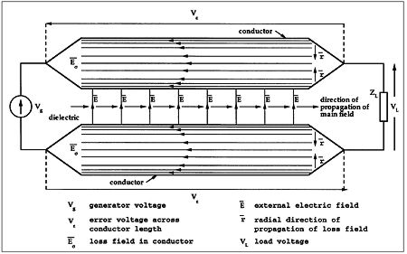 Fig.4 Basic field relationships and direction of propagation of main external field and internal loss field.
The "Ohm's Law" of Maxwell's Equations states J-Barσ = σE-Barσ, which indicates that a conduction current density J-Barσ is induced axially within the conductors due to the internal electric field E-Barσ of the loss wave. This axial current is the current we normally associate with cables—the model we have developed is compatible with the more usual observations of cable behavior. Since the electromagnetic energy of the loss wave propagates principally in a radial direction and enters the conductor over its surface area, the current density (proportional to E-Barσ) is greatest at the surface, and decays as the field propagates into the conductor interior. It is this reason why a conductor experiences a "skin effect" on the outer region rather than the converse situation of current concentrated near the center of the conductor.
Timing problems
Fig.4 Basic field relationships and direction of propagation of main external field and internal loss field.
The "Ohm's Law" of Maxwell's Equations states J-Barσ = σE-Barσ, which indicates that a conduction current density J-Barσ is induced axially within the conductors due to the internal electric field E-Barσ of the loss wave. This axial current is the current we normally associate with cables—the model we have developed is compatible with the more usual observations of cable behavior. Since the electromagnetic energy of the loss wave propagates principally in a radial direction and enters the conductor over its surface area, the current density (proportional to E-Barσ) is greatest at the surface, and decays as the field propagates into the conductor interior. It is this reason why a conductor experiences a "skin effect" on the outer region rather than the converse situation of current concentrated near the center of the conductor.
Timing problems
One of the more informative parameters that we can calculate is the time Tδ; for the sinusoidal loss field Eσ to traverse a distance δ within a good conductor, where, since
v = ω/β = ω/α = ωδ
then
Tδ = δ/v = 1/ω, as long as σ is very much greater than ωε.
For example, consider a copper bar whose diameter is very much greater than its skin depth:
δ = 0.66mm at 10kHz: Tδ = 15.9µs
δ = 2.09mm at 1kHz: Tδ = 0.159ms
δ = 6.61mm at 100Hz: Tδ = 1.59ms
For conductor diameters that are very much greater than the skin depth, Tδ increases with decreasing frequency—there is energy storage; it is a memory mechanism. The model we have developed attempts to show that a good but unnecessarily large conductor influences transient behavior by time-smearing a small fraction of the applied signal by a significant amount.
Consider the cable construction shown in fig.4, where the generator inputs a sinewave for a time very much greater than Tδ, enabling the steady-state to be attained. The E-Bar field between the conductors responds rapidly to the applied signal, as the velocity in the dielectric between the conductors is very high. (We are assuming here a terminating load to the cable, so there is a net energy flow through the dielectric.) As the wavefront progresses, a radial loss wave propagates into each conductor, where the E-Barσ field is aligned in an axial direction.
Now allow the applied signal to be suddenly switched off. The field between the conductors collapses rapidly, thus cutting off the signal energy being fed radially into the conductors. However, the low velocity and high attenuation of the loss wave represents a lossy-energy reservoir, where the time for the wave to decay to insignificance as it propagates into the interior of the conductor is nontrivial by audio standards. The E-Barσ field within the conductor can be visualized as many "strands" of the E-Bar field, as shown in fig.4.
The error voltage, Vint, appearing across the ends of each thread due to the internal conductor impedance, is calculated by multiplying the E-Barσ field by the cable length L (though strictly this should be an integral performed over each elemental length of the cable). Because the field propagates slowly, this summation is actually an average taken over a time window that extends over a short history of the loss field. Consequently, when the generator stops, the error signal across each conductor does not collapse instantaneously. Instead, the conductor momentarily becomes the generator, and a small time-smeared transient residual occurs as the locally stored energy within each conductor dissipates to insignificance. To this voltage must be added the generally more dominant induced voltage, Vext, arising from the changing external magnetic field. Together, they constitute an error voltage Vε = Vint + Vext. Assuming the two conductors are symmetrical, then the load voltage VL is related to the generator voltage Vg by VL = Vg–2Vε.
Although Vε is very much smaller than Vg, the error voltage can take on a complicated and time-smeared form that in practice is both a function of the conductor geometry, cable characteristic impedance, generator source impedance, and load impedance, as all these factors govern the propagation of both the main field E-Bar and loss field E-Barσ.
In practice, unless the cable is terminated in its characteristic impedance, the external field E-Bar residing in the dielectric will traverse the length of the cable rapidly back and forth many times before establishing a pseudo-steady state. Even an optimal load termination implies a significant loss field in the conductors. This argument would suggest that for non–power-carrying interconnects, it is better to terminate the generator end of the cable in the characteristic impedance, leaving the load as a high impedance. The E-Bar field is then rapidly established in the dielectric without either multiple reflection along the cable length, or a finite power flow to the load spilling out a loss wave into the conductors.
Theory vs measurement
Let us now consider an experiment with measurements performed on an actual cable to see whether we can observe the error predicted from theory when the signal stops abruptly. Fig.5 shows a measurement system used to determine the error voltage due to the internal fields of a folded loop of steel wire. (The diameter of the wire is 2.6mm, approximately 0.1".) The folded conductors are insulated but squeezed closely together to minimize the external magnetic field, hence the cable inductance. However, there will still be a residual external magnetic flux, so electronic compensation is made using a differentiator. This enables the signal to be subtracted from the voltage produced at the ends of the loop.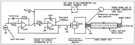 Fig.5 Measurement system for extracting error signal due to internal loss field within a conductor exhibiting significant "skin" depth.
Note that the series inductance due to the external magnetic field produces a voltage proportional to the rate of change of magnetic flux (in turn proportional to the current). By subtracting the correct proportion of this voltage, therefore, the error voltage due to the internal fields in the conductor will be revealed. This supports the idea of measuring the actual error of a specific mechanism rather than letting it become swamped by a higher-level component.
Fig.6 shows a computer simulation of a toneburst that has been modified by a transfer function similar to that occurring in the cable. A similar measured result is shown in fig.7. In the steady state, a 45° phase shift occurs. However, after the tone is switched off a dispersive component is revealed. This latter period is where the energy contained within the conductors decays and is constrained by the low velocity of propagation within a good conductor.
Fig.5 Measurement system for extracting error signal due to internal loss field within a conductor exhibiting significant "skin" depth.
Note that the series inductance due to the external magnetic field produces a voltage proportional to the rate of change of magnetic flux (in turn proportional to the current). By subtracting the correct proportion of this voltage, therefore, the error voltage due to the internal fields in the conductor will be revealed. This supports the idea of measuring the actual error of a specific mechanism rather than letting it become swamped by a higher-level component.
Fig.6 shows a computer simulation of a toneburst that has been modified by a transfer function similar to that occurring in the cable. A similar measured result is shown in fig.7. In the steady state, a 45° phase shift occurs. However, after the tone is switched off a dispersive component is revealed. This latter period is where the energy contained within the conductors decays and is constrained by the low velocity of propagation within a good conductor.
 Fig.6 Predicted error due to internal loss field of conductor operating in skin depth-limited region.
 Fig.7 Measured error due to internal loss field of conductor operating in skin depth-limited region. Note that input and output waveforms are not on the same scale, and that time dispersion is proportional to the tone period in the skin depth-limited region, meaning that the time scale is immaterial.
Fig.3 Cross-section of coaxial cable showing radial E-Bar field and circumferential H-Bar field.
Power flow
In an electromagnetic system, the "power flow" is a directed or vector quantity and is represented as a power-density function P-Bar (watt/m2) called the Poynting Vector, where P-Bar = E-Bar x H-Bar (with x being the vector crossproduct rather than the conventional multiplication symbol). For a coaxial cable, P-Bar is directed axially, indicating that energy is propagated along the cable. Integrate P-Bar over a cross-section of area (between the conductors) and the result is the total power carried by the cable. The expression for P-Bar can be compared with power calculations in lumped electrical systems, where P (power) = V (voltage) x I (current) (ie, V is equivalent to the E-Bar field, I to the H-Bar field).
Fig.4 Basic field relationships and direction of propagation of main external field and internal loss field.
The "Ohm's Law" of Maxwell's Equations states J-Barσ = σE-Barσ, which indicates that a conduction current density J-Barσ is induced axially within the conductors due to the internal electric field E-Barσ of the loss wave. This axial current is the current we normally associate with cables—the model we have developed is compatible with the more usual observations of cable behavior. Since the electromagnetic energy of the loss wave propagates principally in a radial direction and enters the conductor over its surface area, the current density (proportional to E-Barσ) is greatest at the surface, and decays as the field propagates into the conductor interior. It is this reason why a conductor experiences a "skin effect" on the outer region rather than the converse situation of current concentrated near the center of the conductor.
Timing problems
One of the more informative parameters that we can calculate is the time Tδ; for the sinusoidal loss field Eσ to traverse a distance δ within a good conductor, where, since
Let us now consider an experiment with measurements performed on an actual cable to see whether we can observe the error predicted from theory when the signal stops abruptly. Fig.5 shows a measurement system used to determine the error voltage due to the internal fields of a folded loop of steel wire. (The diameter of the wire is 2.6mm, approximately 0.1".) The folded conductors are insulated but squeezed closely together to minimize the external magnetic field, hence the cable inductance. However, there will still be a residual external magnetic flux, so electronic compensation is made using a differentiator. This enables the signal to be subtracted from the voltage produced at the ends of the loop.
Fig.5 Measurement system for extracting error signal due to internal loss field within a conductor exhibiting significant "skin" depth.
Fig.6 Predicted error due to internal loss field of conductor operating in skin depth-limited region.
Fig.7 Measured error due to internal loss field of conductor operating in skin depth-limited region. Note that input and output waveforms are not on the same scale, and that time dispersion is proportional to the tone period in the skin depth-limited region, meaning that the time scale is immaterial.