Wilson Audio Specialties Alexia loudspeaker Measurements

Sidebar 3: Measurements

I used DRA Labs' MLSSA system and a calibrated DPA 4006 microphone to measure the Wilson Alexia's frequency response in the farfield, and an Earthworks QTC-40 for the nearfield and spatially averaged room responses. Because of the speaker's bulk, I was unable to raise it off the ground for the measurements; this will reduce the resolution of the frequency-response graphs in the midrange. Then there was the problem of which axis to place the microphone on for the farfield measurements. Yes, the way the tweeter module is mounted atop the midrange module facilitates repeatability in adjusting its position, but I wanted to measure the speaker as it had been set up by Wilson's Peter McGrath. I also wanted to measure it at my standard 50" microphone distance, which is optimal for midrange resolution in the resultant graphs, even with the speaker on the floor. So I drew a line from the tweeter to the 36" height of my ears, 106" away, then moved the mike up along that line until it was 50" from the tweeter. Other than those used to assess the Alexia's vertical dispersion, all the farfield measurements were taken at that point.

My estimate of the Alexia's voltage sensitivity was slightly higher than the specified 90dB/2.83V/m, at 91.3dB(B)/2.83V/m. This speaker will play loudly with just a few watts. However, it demands quite a lot of current from the partnering amplifier. The Alexia's electrical impedance and phase angle are shown in fig.1. (This graph was taken with the original, higher-value tweeter resistors.) The impedance magnitude stays between 2 and 6 ohms from 12Hz to 4kHz, with a gentle rise above that frequency. The minimum value is 1.96 ohms at 86Hz, and there is a demanding combination of 3.6 ohms and –43° phase angle at 54Hz.

1213Walexfig01.jpg

Fig.1 Wilson Alexia, electrical impedance (solid) and phase (dashed) (2 ohms/vertical div.).

The traces in fig.1 are free from the small glitches that would hint at the presence of vibrational resonances in the enclosures. Looking for the existence of such resonances with a simple plastic-tape accelerometer (similar to a piezoelectric guitar pickup), I could find nothing on the woofer enclosure. I did discover some modes on the walls of the midrange enclosure (fig.2), but these are very low in level; I am confident in saying that they will have no effect on sound quality.

Walexfig02.jpg

Fig.2 Wilson Alexia, cumulative spectral-decay plot calculated from output of accelerometer fastened to center of midrange-enclosure side panel (MLS driving voltage to speaker, 7.55V; measurement bandwidth, 2kHz).

The fact that the binding posts for the tweeter and midrange unit are accessible allowed me to examine the farfield acoustic crossover on the listening axis. Fig.3 reveals that the crossover between the tweeter (black trace) and the midrange unit (green) is set at a low 1.5kHz. Though some cone-breakup modes are evident in the midrange unit's output more than a couple of octaves above the crossover point, these are well suppressed by the low-pass filter. The tweeter's output is basically flat within its passband, and extends at full level to the 30kHz limit of this graph. However, a narrow suckout is visible between 4 and 5kHz, this perhaps arising from destructive interference between the tweeter's direct output and the reflections from the midrange enclosure.

Walexfig03.jpg

Fig.3 Wilson Alexia, acoustic crossover on listening axis at 50", corrected for microphone response, with nearfield responses of: midrange unit (green), woofers (blue), port (red), respectively plotted below 350Hz, 1kHz, 300Hz.

To the left in fig.3 are shown the nearfield outputs of the midrange unit (green), the woofers (blue), and the port that loads the woofers (red). (Though they have different radiating diameters, the two woofers behave virtually identically, so I have shown the sum of their outputs.) The midrange unit has a very wide passband; it slopes down a little throughout the midrange, before crossing over to the woofers around 150Hz. For clarity, I haven't shown the nearfield output of the twin slots that load the midrange unit; they don't extend the unit's output, but, as in other Wilson speakers, act to increase its dynamic-range capability at the bottom of its passband. The woofers cover a narrow passband, though this is visually exaggerated in fig.3 by the usual boost in the upper bass that results from the nearfield measurement technique. They roll off above 150Hz with what appears to be a second-order slope, and have a sharply defined notch in the low-bass output at the low port tuning frequency of 23.5Hz. The port's output covers a wider range than usual but rolls off rapidly above 70Hz, with no resonant modes visible.

Fig.4 shows how these individual responses sum in the farfield, averaged across a 30° horizontal window centered on the listening axis. The response is impressively flat throughout the upper midrange and treble, though that small suckout between 4 and 5kHz is still apparent. There is a slight lack of energy in the lower midrange where the outputs of the woofers and midrange unit slightly overlap. The peak in the midbass is entirely due to the nearfield measurement technique. The Alexia appears to have a slightly overdamped reflex alignment, which results in its nearfield output being down by 12dB at 20Hz. However, as the speaker's low-bass output will be reinforced by boundary reflections in all but very large rooms, this alignment optimizes low-frequency clarity without sacrificing effective bass extension. Very sensible.

Walexfig04.jpg

Fig.4 Wilson Alexia, anechoic response on listening axis at 50", averaged across 30° horizontal window and corrected for microphone response, with complex sum of nearfield responses plotted below 300Hz.

If you compare the traces above 20kHz in figs. 3 and 4, you can see that the averaged response is more rolled off than the listening-axis response. This is because, as can be seen in the plot of the Alexia's lateral dispersion (fig.5), the tweeter becomes very directional above 12kHz or so. The apparent off-axis peak between 4 and 5kHz in this graph is due to that on-axis suckout noted earlier filling in to the speaker's sides. The same is true for the small depression in the on-axis response between 1 and 2kHz. Overall, the Alexia's off-axis behavior is well controlled and even, at least up to the point where the tweeter becomes directional. In the vertical plane (fig.6), a sharp suckout develops at the upper crossover point more than 5° above the listening axis, but the speaker otherwise appears relatively unfussy. There is nothing to suggest why I felt that moving my ears slightly above or below the listening axis introduced a narrow band of brightness, as mentioned in the "Listening" section of this review.

Walexfig05.jpg

Fig.5 Wilson Alexia, lateral response family at 50", normalized to response on listening axis, from back to front: differences in response 90–5° off axis, reference response, differences in response 5–90° off axis.

Walexfig06.jpg

Fig.6 Wilson Alexia, vertical response family at 50", normalized to response on listening axis, from back to front: differences in response 15–5° above axis, reference response, differences in response 5–10° below axis.

The blue trace in fig.7 shows the spatially averaged response of the Alexias in my listening room, fitted with the original 4.5 ohm series resistors in the tweeter feeds. (The trace was generated by averaging 20 1/6-octave–smoothed spectra, taken for the left and right speakers individually using SMUGSoftware's FuzzMeasure 3.0 program and a 96kHz sample rate, in a vertical rectangular grid 36" wide by 18" high and centered on the positions of my ears.) As I mentioned, I felt that the Alexia lacked a little top-octave air in my room, so Wilson sent me substitute 3.5 ohm resistors to increase the output of the tweeters. The in-room response with these resistors is shown as the red trace in fig.7. You can see that the change increased the level of the region covered by the tweeter by approximately 1dB.

Walexfig07.jpg

Fig.7 Wilson Alexia, spatially averaged, 1/6-octave response in JA's listening room with: original tweeter resistors (blue), new tweeter resistors (red). Note expanded vertical scale compared with fig.8.

The vertical scale in fig.7 has been exaggerated to emphasize the difference made by the tweeter resistors. The red trace in fig.8 repeats the in-room response of the Alexias with the new tweeter resistors, plotted with my usual scaling. For reference, the blue trace in this graph shows the spatially averaged response of YG Acoustics' Sonja 1.3, which I reviewed in July. This kind of in-room response should gently slope down with increasing frequency, due to the increasing absorptivity of the room furnishings at high frequencies, and that is what the Alexias do. The YGAs had a little too much energy in the mid- and high-treble regions, the Wilsons a little too much presence-region energy; the latter may well correlate with their superb retrieval of recorded detail. Though both speaker models have two spaced woofers, the Sonja 1.3 deals better with the "floor-bounce" region in the lower midrange. The Alexia, however, has a more even output in the bass, with more energy apparent in its port-tuning region below the frequency of the lowest mode in my room.

1213Walexfig08.jpg

Fig.8 Wilson Alexia, spatially averaged, 1/6-octave response in JA's listening room with new tweeter resistors (red); and of YG Acoustics' Sonja 1.3 (blue).

In the time domain, the Alexia's step response on its listening axis is shown in fig.9. This graph reveals that, as in the Alexandria XLF, the tweeter is connected in positive acoustic polarity, the midrange driver in negative polarity. However, with the tweeter module set up by Peter McGrath, the graph also shows that the negative-going decay of the tweeter's step smoothly blends with the negative-going start of the midrange unit's step, confirming the excellent frequency-domain integration of their outputs seen in fig.4. Moving slightly above or below the intended axis destroys that smooth blending of step responses. Fig.9 also reveals that the woofers are both connected in positive acoustic polarity (confirmed by their nearfield step responses, not shown), with, at this too-close distance, the upper woofer's output clearly arriving at the mike before the lower woofer's. The cumulative spectral-decay plot on this axis (fig.10) did not look as clean as I was expecting. There is a minor ridge of delayed energy around 15kHz, this coincident with a small, narrow notch in the on-axis response, but this will be benign.

1213Walexfig09.jpg

Fig.9 Wilson Alexia, step response on listening axis at 50" (5ms time window, 30kHz bandwidth).

1213Walexfig10.jpg

Fig.10 Wilson Alexia, cumulative spectral-decay plot on listening axis at 50" (0.15ms risetime).

Overall, the Alexia measures well. Its Aspherical Group Delay feature appears to be effective at optimizing its performance at the height of the listener's ears—not only in the time domain, but also, I conjecture, in adjusting the frequency and depth of that small mid-treble suckout in the direct response to have minimal effect on the music.—John Atkinson

COMPANY INFO
Wilson Audio Specialties
2233 Mountain Vista Lane
Provo, UT 84606
(801) 377-2233
ARTICLE CONTENTS

COMMENTS
Regadude's picture

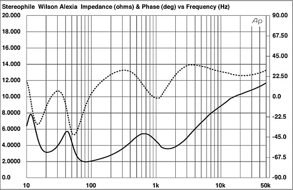
Really, no comments? Last year when the 200K Wilson's were reviewed, the comments section went crazy! So many people (who had never heard the Wilsons) were angry and torched the product. Some judged the speakers only on the measurements... And, they went ballistic!

No measurements were done for this review. Also, no comments. What a difference a year makes!

John Atkinson's picture

Regadude wrote:
No measurements were done for this review.

No measurements? Check out www.stereophile.com/content/wilson-audio-specialties-alexia-loudspeaker-measurements.

John Atkinson
Editor, Stereophile

billyjul's picture

this loudspeaker is not high-end , except if you look the price only, beacause the main concept has som flaws, that drivers whith exotic sanswich cône whtih cabon nanotube, diamond, roacel, or other matérials  witch cost a fortune can't change

the main concept of this speaker stay the same

you can realise a speaker using the kinoshita concept, used in rey audio monitor ou or tad loudspeaker, and sold a fraction of the alexia price, whith really excelent 15" drivers from PHL audio, TAD or JBL, and a 2" compresion coaxial BMS4590 with it's horn BMS2236 

it will do better beacause the main concept is better

that's all

Regadude's picture

I have never heard this speaker, so I won't offer an opinion on its sound quality. But, I find that bright orange paint job just a little too much. 

They do look extremely well built though. I would be curious to hear them, but it's probably better that I didn't. The problem with going to shows and hearing 40 000$ speakers, is that it takes a few days for your own system to start sounding good again!

georgehifi's picture

HIFI NEWS has a added measured spec, that should be included.

http://www.absolutesounds.com/pdf/main/press/WA%20Alexia%20HFN%200313-4web.pdf

The combind phase and impedance (EPDR) at 65hz is evil, not stated in the Stereophile measurements.

It represents a load of .9 of an ohm. To get the best out of the bass around this frequency you need bags of current, tubes and mosfet output stages need not apply.

You need a good big solid state amp that has a BJT (bi-polar) output stage that can dump heaps of current into this to get the best bass out of these. 


Cheers George  

John Atkinson's picture

Georgehifi wrote:
HIFI NEWS has a added measured spec, that should be included.

http://www.absolutesounds.com/pdf/main/press/WA%20Alexia%20HFN%200313-4web.pdf

The combind phase and impedance (EPDR) at 65hz is evil, not stated in the Stereophile measurements. It represents a load of 0.9 of an ohm.

The Alexias have long since been returned to Wilson but I reexamined the raw data I used to plot fig.1 in my review. At 65.5Hz the impedance was 2.26 ohms with a phase angle of   -30.5 degrees. The largest phase angle was -42.25 degrees at 53Hz, but the impedance magnitude at that frequency was 3.7 ohms.

HFN's minimum impedance was 1.8 ohms at 85Hz; mine was I.97 ohms at 83Hz, though my measurement does includes the series resistance of 10' of speaker cable, which might explain the small difference. .

Why the discrepancy between my measurement and Keith Howard's for HiFi News? Different samples, of course, but also different measurement techniques: Keith uses DRA Labs' MLSSA, which produces an FFT-derived result and also compensates for the speaker cable resistance, while I use a swept series of spot-frequency tones using an Audio Precision System One. I check my findings by measuring the impedance of a 10 ohm resistor; there didn't appear to be anything untoward with my measurement of the Alexia.

When I get home this evening, I will check Martin Colloms' impedance measurement in The HiFi Critic.

John Atkinson

Editor, Stereophile

John Atkinson's picture

John Atkinson wrote:
When I get home this evening, I will check Martin Colloms' impedance measurement in The HiFi Critic.

Okay, Martin describes the Alexia's impedance on p.15 of the Jan/Feb/Mar 2013 issue. His impedance curves (on p.17) look very similar to my fig.1. His minimum impedance was 1.8 ohms at 80Hz with a -20 degree phase angle and he also mentions the impedance at 60Hz as being 2.5 ohms with a -42 degree phase angle. (Martin uses the Clio system for his speaker measurements.)

So neither Martin's nor my measurements indicate that the Alexia's impedance is quite as punishing as Keith's, though yes, the Alexia _must_ be driven by an amplifier that isn't fazed by low impedances. As I wrote in my review, the Alexia "demands quite a lot of current from the partnering amplifier."

John Atkinson

Editor, Stereophile

nile49's picture

Hi John,

I was wondering if you could comment on the EPDR calculation mentioned above. Why don't you don't use it? Does this method of calculation have potential pitfalls? Etc.

It seems to me to be a very clear and easy way to compare and to understand otherwise tricky to interpret measurements.

Thanks, Warren

John Atkinson's picture

nile49 wrote:
I was wondering if you could comment on the EPDR calculation mentioned above. Why don't you don't use it?

Including it in my published speaker measurements has been on my To-Do list for several years. I wanted to kickoff using it by applying the calculation retroactively to every loudspeaker I have measured for Stereophile and publish the results in an article. But like all things that are important but not urgent, it gets push back and back and back. . . :-(

John Atkinson

Editor, Stereophile

Chopin's picture

I don’t Know M Atkinson how you make your measurement ??
You say 91.3 db 2.83 v/m........habitually 2.83 volts 1 watts / 1 meter is for 8 ohms loudspeaker.
The loudspeaker have near of 2 ohms ?? It,s sure if you put 2.83 volts in 2 ohms you will have 4 watts
To have 1 w 1 m at 2 ohms you will put 1.41 volts . Don’t forget amp with 2 ohms should less stable.
Bizarre ???

John Atkinson's picture
Chopin wrote:
You say 91.3 db 2.83 v/m........habitually 2.83 volts 1 watts / 1 meter is for 8 ohms loudspeaker. The loudspeaker have near of 2 ohms ?? It,s sure if you put 2.83 volts in 2 ohms you will have 4 watts

That is correct, but I don't measure sensitivity in db/W but dB/V, the voltage sensitivity. This is because amplifiers are voltage sources; see www.stereophile.com/content/measuring-loudspeakers-part-one-page-3.

John Atkinson
Editor, Stereophile

X