Sumo Axiom CD transport & Theorem II D/A processor Measurements

Sidebar 2: Measurements

The Theorem II's maximum output level was 2.03V, conforming with the CD standard of 2V output. The output impedance was a low 70 ohms at 20Hz, decreasing to 50 ohms at 1kHz and above, making the Theorem II insensitive to preamplifier loading. DC levels were negligible, measuring just 0.2mV (left channel) and 0.1mV (right channel). The Theorem II's polarity button works: set to positive polarity, the Sumo doesn't invert absolute polarity from its RCA outputs. Because pin 2 of the XLR connector is the signal conductor and pin 3 is grounded, the Theorem II will be non-inverting from the XLR outputs when connected to other pin-2–hot equipment. The Theorem had no trouble decoding 32kHz and 48kHz sampling frequencies.

Fig.1 shows the Theorem II's frequency response and de-emphasis error. The response shows a typical mild top-octave rolloff, and the analog-domain de-emphasis circuit is accurate, meaning you won't hear a tonal balance difference when playing the few pre-emphasized CDs you may have. The Theorem II's plot of channel separation is shown in fig.2. The left/right-channel crosstalk is slightly lower than the R–L above 800Hz, and meets the claimed !w80dB separation specification; crosstalk in the other direction does not.

666thSumo2fig01

Fig.1 Sumo Theorem II, frequency response (top) and de-emphasis error (bottom) (right channel dashed, 0.5dB/vertical div.).

666thSumo2fig02

Fig.2 Sumo Theorem II, R–L crosstalk in balanced mode (L–R dashed, 10dB/vertical div.).

A spectral analysis of the Theorem II's output with the unit decoding a 1kHz, –90dB dithered sinewave (fig.3) shows some problems. First, we can see a moderately high noise level. Second, the trace peaks above the –90dB horizontal division, indicating a positive linearity error. Third, the peak at 2kHz indicated that the Theorem II's DAC is creating second-harmonic distortion, particularly in the left channel. [This is normally due to low-level non-monotonicity in the DAC.—Ed.] Finally, we can see power-supply noise as peaks at 60Hz, 120Hz, 180Hz, and 300Hz. This amount of power-supply noise in the audio circuitry isn't severe; even the worst component (60Hz, right channel) is more than 105dB down and should be inaudible. Nonetheless, this spectral analysis plot is not ideal.

666thSumo2fig03

Fig.3 Sumo Theorem II, spectrum of dithered 1kHz tone at –90.31dBFS, with noise and spuriae (1/3-octave analysis, right channel dashed).

Performing the same test, but increasing the bandwidth to 200kHz and driving the Theorem II with all zeros, produced the plot of fig.4. Unusually for a noise-shaping DAC, there's no significant rise in the noise floor above the audioband.

666thSumo2fig04

Fig.4 Sumo Theorem II, spectrum of digital silence (1/3-octave analysis, right channel dashed).

The Theorem II's linearity error is more apparent in fig.5. We can see 4dB of positive error at –90dB (right channel)—a significant departure from linearity by today's standards. Fig.6 is the Theorem II's reproduction of a 1kHz, –90dB undithered sinewave. The waveform looks unusual in that it should be symmetrical. Instead, the "0" levels appear as the steps at the 50µV division; the "+1" step peaks at the 100µV division, and the "–1" step is all the way down at –200µV. This uneven step size is so severe that it's hard to distinguish between the 0 and +1 levels. I was surprised by this aspect of the Theorem II's performance, because the PCM69 DAC uses a 1-bit converter for the lower eight bits, which should have better low-level performance than is indicated by this waveform. This behavior does correlate, however, with the spectral analysis in fig.3.

666thSumo2fig05

Fig.5 Sumo Theorem II, departure from linearity (right channel dashed, 2dB/vertical div.).

666thSumo2fig06

Fig.6 Sumo Theorem II, waveform of undithered 1kHz sinewave at –90.31dBFS.

As might be expected, the noise-modulation performance (fig.7) was also poor. The Theorem II showed large shifts in the noise floor as a function of input level. In fact, the noise floor shifts as much as 4dB through most of the audioband as the input level changes—not a good thing. Because very few of the traces don't cross each other, the noise floor's spectral balance remains constant, but the level shift is substantial.

666thSumo2fig07

Fig.7 Sumo Theorem II, noise modulation, –60 to –100dBFS (10dB/vertical div.).

So far, we have looked at low-level idiosyncrasies. How about at the other end of the dynamic range scale? Fig.8 shows an FFT-derived spectral analysis of the Theorem II's output while it decodes data representing a full-scale mix of 19kHz and 20kHz tones. We can see an entire series of intermodulation components as the spikes at 1kHz intervals. Although all are fairly low in level (below –95dB), the number of IMD components is high.

666thSumo2fig08

Fig.8 Sumo Theorem II, HF intermodulation spectrum, DC–22kHz, 19+20kHz at 0dBFS (linear frequency scale, 20dB/vertical div.).

The separate clock link between the Theorem II and the Axiom made it possible to measure the difference in jitter performance with and without the clock link. In addition, I measured the Theorem II's clock jitter when driven by the Axiom transport and the PS Audio Lambda transport. First, I measured the Theorem II's jitter performance with the Meitner LIM Detector, using the PS Audio Lambda transport to play test tones on the CBS Test Disc. (For consistency, we use the Lambda transport and the same digital interconnect in all our jitter measurements.)

Fig.9 is the Theorem II's word-clock jitter, measured at the 8x-oversampling "WCLK" pin on the PCM69 DAC, with a 1kHz, 0dBFS sinewave input signal. We can see a predominant spike at the test-signal frequency, and also a large number of discrete-frequency jitter components. This trace looks poor, indicating lots of periodic jitter on the clock at many frequencies. The RMS jitter level, measured over a 400Hz–22kHz bandwidth, was a whopping 1150ps (1.15ns). When the Theorem II was driven by a 1kHz sinewave at –90dB, the jitter spectrum showed spikes at 1kHz and 2kHz, but was cleaner overall (fig.10). The RMS level, however, increased to 1950ps (nearly 2ns). The spike at 7.35kHz is the subcode data rate within the S/PDIF interface.

666thSumo2fig09

Fig.9 Sumo Theorem II, word-clock jitter spectrum, DC–20kHz, when processing 1kHz sinewave at 0dBFS, PS Audio Lambda transport (linear frequency scale, 10dB/vertical div., 0dB=1ns).

666thSumo2fig10

Fig.10 Sumo Theorem II, word-clock jitter spectrum, DC–20kHz, when processing 1kHz sinewave at –90dBFS, PS Audio Lambda transport (linear frequency scale, 10dB/vertical div., 0dB=1ns).

Fig.11 is the Theorem II's jitter, again driven by the Lambda transport, but now with an input signal of all zeros. Again, the large spike at 7.35kHz is the subcode data rate, but the number of periodic jitter components has changed again. However, the RMS jitter level dropped to a still-high 575ps. These are very large differences in jitter performance as the input signal changes.

666thSumo2fig11

Fig.11 Sumo Theorem II, word-clock jitter spectrum, DC–20kHz, when processing digital silence, PS Audio Lambda transport (linear frequency scale, 10dB/vertical div., 0dB=1ns).

I repeated these measurements using the Axiom as the transport without the clock link engaged. We can assume that if the Theorem II's clock jitter drops with the Axiom, the Sumo transport has lower intrinsic jitter than that of the PS Audio Lambda. If the Theorem II's word-clock jitter increases, the Axiom has higher jitter than that of the Lambda.

Fig.12 is the Theorem II's jitter with the Axiom transport playing a 1kHz, 0dBFS sinewave. It looks about the same as with the Lambda, but the RMS jitter level increased to 1440ps (compared to 1150ps with the Lambda). More illustrative is the Theorem II's jitter when the unit is decoding a 1kHz, –90dB sinewave (fig.13). Comparing fig.10 (with the Lambda) to fig.13 (with the Axiom), we see many more periodic jitter components, and a slightly higher RMS jitter level (2370ps), in the Theorem II when it's driven by the Axiom. With an input of all zeros, the Axiom transport produced a very slightly cleaner spectrum than did the Lambda (not shown), but the RMS level was 680ps with the Axiom (compared to 575ps with the Lambda).

666thSumo2fig12

Fig.12 Sumo Theorem II, word-clock jitter spectrum, DC–20kHz, when processing 1kHz sinewave at 0dBFS, Sumo Axiom transport but no clock link (linear frequency scale, 10dB/vertical div., 0dB=1ns).

666thSumo2fig13

Fig.13 Sumo Theorem II, word-clock jitter spectrum, DC–20kHz, when processing 1kHz sinewave at –90dBFS, Sumo Axiom transport but no clock link (linear frequency scale, 10dB/vertical div., 0dB=1ns).

The Theorem II's measured jitter performance improved dramatically when the Theorem II was locked to the Axiom by the separate clock line. Fig.14 is the Theorem II's jitter with a 1kHz, 0dBFS sinewave input. Note the vastly lower number of periodic jitter components (fewer spikes in the plot). In addition to producing a cleaner jitter spectrum, the RMS jitter level dropped more than an order of magnitude, to just 120ps (compared to 1440ps without the clock link). There seems to be a clear correlation here between my listening experiences and the measured jitter performance. Apparently, reducing the jitter from 1440ps to 120ps and making the jitter more random has a large effect on sound quality, as noted in the auditioning.

666thSumo2fig14

Fig.14 Sumo Theorem II, word-clock jitter spectrum, DC–20kHz, when processing 1kHz sinewave at 0dBFS, Sumo Axiom transport with clock link (linear frequency scale, 10dB/vertical div., 0dB=1ns).

Fig.15 is the Theorem II's jitter spectrum with the Axiom transport and separate clock link, with an input data representing a 1kHz, –90dB sinewave. Compare this plot with fig.13: the improvement in jitter performance rendered by the clock link is dramatic. The RMS jitter level in fig.15 is 115ps.

666thSumo2fig15

Fig.15 Sumo Theorem II, word-clock jitter spectrum, DC–20kHz, when processing 1kHz sinewave at –90dBFS, Sumo Axiom transport with clock link (linear frequency scale, 10dB/vertical div., 0dB=1ns).

Finally, fig.16 is the Theorem II's jitter when connected to the Axiom with the clock link and an input signal of all zeros. The trace is very clean, and almost as good as it gets. The RMS jitter level dropped to a very low 75ps. Sumo claims the Theorem II's jitter to be !x80ps—a figure just met by this last condition (Axiom transport, clock link, input of all zeros). Note, however, that there are no standards for how and under what conditions (such as input signal, measurement bandwidth, peak or RMS, and many other factors) jitter measurements are made.

666thSumo2fig16

Fig.16 Sumo Theorem II, word-clock jitter spectrum, DC–20kHz, when processing digital silence, Sumo Axiom transport with clock link (linear frequency scale, 10dB/vertical div., 0dB=1ns).

We can draw several conclusions from these measurements. First, the transport driving the Theorem II affects its clock jitter, and thus its sound. Moreover, the Axiom appears to have higher intrinsic jitter than the Lambda. The wide variation in the Theorem II's jitter level and spectrum as the input signal was varied suggests that this processor is highly sensitive to interface jitter, and will thus be more transport-sensitive than other processors. (I did hear a significant improvement in the sound when the Theorem was driven by the Mark Levinson No.31 rather than the Axiom.) Finally, the Theorem II's vastly lower jitter when connected to the Axiom with the separate clock line reinforces the validity of this technique, and also suggests that the Axiom and Theorem should be used together for best performance—another conclusion suggested by the auditioning.

Overall, the Theorem II had only fair to poor bench performance. Our sample suffered from poor DAC monotonicity, as revealed by the production of second-harmonic distortion, poor low-level linearity, uneven step size when reproducing low-level signals, and shifts in the noise floor as a function of input level.—Robert Harley

COMPANY INFO
Sumo Products Group
Company no longer in existence (2019)
ARTICLE CONTENTS

COMMENTS
hollowman's picture

As was done recently with orig. 1987 PS Audio DAC, Stereophile should re-review the gear if possible. Ask for loaners on FB or the forums as needed.
New product developers and customers need some sort of "reference metric". E.g., how much has digital technology improved ... subjectively and objectively (measurements).

JRT's picture

For more than two decades, you have been able to rip once, play many, and do so with more precision and accuracy and consistency than with any real time CDP.

Playback using physical media is archaic, regardless if CD, LP or 8-track tape cassettes.

Ortofan's picture

... start with this unit:
https://www.stereophile.com/content/sony-cdp-x779es-cd-player
The measured performance was outstanding and JGH said he'd buy one.

Bogolu Haranath's picture

Bryston BCD-3 ($3,500) measurements are comparable to the Sony CDP-X779 ES :-) ........

Bogolu Haranath's picture

Maranz CD 5005 ($400) and CD 6006 ($500) could offer similar excellent measurements as the Sony and Bryston CD players :-) .........

Bogolu Haranath's picture

Stereophile could review the Denon DCD-600NE ($300) CD player :-) .........

Bogolu Haranath's picture

Adjusted for inflation the Sony CDP-X779 ES would cost approximately $4,000 in 2019 :-) ........

X