Floor Loudspeaker Reviews

Kalman Rubinson waxed lyrical about PSB's surprisingly affordable Image T6 tower loudspeaker in the March 2010 issue of Stereophile. For $1199/pair, you get a well-finished, superb-sounding speaker. "With much more massive music, such as Christoph Eschenbach and the Philadelphia Orchestra's performance of Mahler's Symphony 6 (SACD/CD, Ondine ODE1084-5D)," Kal wrote, "the T6s offered the same deep, spacious, detailed soundstage as they had with the chamber recordings, but on a larger scale. There was such a feeling of effortlessness that I was encouraged to turn up the volume to a near natural level." He concluded that, "for $1199/pair, [the PSB Image T6] is an absolutely wonderful full-range speaker, and is now my quasi-$1000/pair standard for an entry-level high-end loudspeaker."

Intrigued, I asked Kal to ship me all three samples of the T6, so that I could perform on them my standard set of measurements. I used DRA Labs' MLSSA system and a calibrated DPA 4006 microphone for the farfield responses, and an Earthworks QTC-40 for the nearfield. The PSB's sensitivity is specified as 89dB/2.83V/m; my estimate came in at 88.2dB/2.83V/m, which is close. PSB specifies the Image T6's impedance at 6 ohms, with a 4 ohm minimum magnitude. My measurement (fig.1) went a little lower than 4 ohms, with a minimum value of 3.1 ohms at 415Hz, and there is also a combination of 4.5 ohms and a –45° electrical phase angle at 94Hz. While the impedance does remain at or above 6 ohms above 1100Hz, this speaker really will work best with amplifiers or receivers rated at 4 ohms.

Fig.1 PSB Image T6, electrical impedance (solid) and phase (dashed). (2 ohms/vertical div.)

The small wrinkles at 26kHz in the fig.1 traces suggest that this is the frequency of the metal-dome tweeter's primary "oil-can" resonance, which is safely above the audioband. The traces are free from the small discontinuities that would indicate the presence of cabinet resonances of various kinds, but investigating the panels' vibrational behavior did uncover a relatively severe mode at 262Hz (fig.2). This was highest in level on the side panels near the speaker's base, but lower-level modes were present on the other surfaces at 234 and 277Hz. I would have expected a degree of lower-midrange congestion to be the result of this behavior, but I note that KR found nothing amiss in this region.

Fig.2 PSB Image T6, cumulative spectral-decay plot calculated from output of accelerometer fastened to center of woofer-enclosure side panel (MLS driving voltage to speaker, 7.55V; measurement bandwidth, 2kHz).

The saddle centered on 41.5Hz in the impedance graph implies that this is the tuning frequency of each of the two ports on the front baffle. The ports had identical outputs, and the woofers were also very closely matched in response. The red trace in fig.3 shows the sum of the two port outputs, which does peak between 30 and 80Hz, with well-controlled rollouts above and below that region. The summed response of the woofers (fig.3, blue trace) has its minimum-motion notch at the port tuning frequency, and their output crosses over to the midrange output (fig.3, green trace) at 550Hz. The crossover appears to be 18dB/octave for the midrange high-pass, and 24dB/octave for the woofers low-pass. The farfield measurements taken to produce this graph were made on the midrange axis, which is 37" from the floor. The output of the midrange and tweeter are extremely flat on this axis, and the inevitable dip below the tweeter resonance doesn't occur until above 19kHz.

Fig.3 PSB Image T6, acoustic crossover on midrange axis at 50", corrected for microphone response, with nearfield responses of woofer (blue) and port (red), plotted below 350Hz and 800Hz, respectively.

Fig.4 shows how these individual drive-unit outputs sum in the farfield, again on the midrange axis. The Image T6's overall response is commendably flat, though there is a slight lack of midrange energy compared with the regions above and below and a slight peak in the mid-treble. Most of the apparent boost in the upper bass will be an artifact of the nearfield measurement technique, but the speaker is balanced a little on the rich side. As I had all three samples available for measurement, I examined each of them. The red trace in fig.5 is the midrange-axis response of the same sample as in fig.4 (S/N 901423); the blue and green traces show the responses of the other two samples (S/Ns 901427 and 901319, respectively). While the tweeter's ultrasonic resonance is a little different in each speaker, overall this is superb matching for what is a reasonably priced model.

Fig.4 PSB Image T6, anechoic response on midrange axis at 50", averaged across 30° horizontal window and corrected for microphone response, with complex sum of nearfield responses plotted below 300Hz.

Fig.5 PSB Image T6, anechoic response on midrange axis at 50", averaged across 30° horizontal window and corrected for microphone response of S/N 901423 (red), 901427 (blue) and 901319 (green).

The Image T6's lateral dispersion on the MF axis is shown in fig.6. The radiation pattern is smooth, even, and well controlled, with just a hint of off-axis flare at the bottom of the tweeter's passband. In the vertical plane (fig.7), there are only mild changes in response as the listener moves above or below the midrange axis.

Fig.6 PSB Image T6, lateral response family at 50", normalized to response on midrange axis, from back to front: differences in response 90–5° off axis, reference response, differences in response 5–90° off axis.

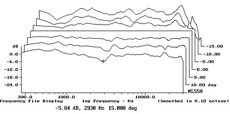
Fig.7 PSB Image T6, vertical response family at 50", normalized to response on midrange axis, from back to front: differences in response 15–5° above axis, reference response, differences in response 5–15° below axis.

In the time domain, the PSB Image T6's step response on the midrange axis (fig.8) indicates that the tweeter and midrange unit are connected in inverted acoustic polarity, the woofers in positive polarity. Reflecting the superb integration of their outputs seen in the frequency domain, the decay of each drive-unit's step is smoothly integrated with the rise of the step of the next lower in frequency. This is textbook design. The PSB's cumulative spectral-decay plot (fig.9) is superbly clean, especially in the tweeter's passband, which is especially commendable at this price level.

Fig.8 PSB Image T6, step response on midrange axis at 50" (5ms time window, 30kHz bandwidth).

Fig.9 PSB Image T6, cumulative spectral-decay plot on midrange axis at 50" (0.15ms risetime).

I am not surprised that Kal Rubinson liked the PSB Image T6 as much as he did. Its measured performance is almost without peer in this price region. This is a speaker you must hear.—John Atkinson