Features

Slope
The third graph in each set will be a complete novelty to most readers. At first glance you might presume it to be a plot of amplitude vs time, just as you would see if you were to view the track in audio editing software (albeit here with the left and right channels superimposed, blue and red traces respectively). But this is actually a graph not of amplitude vs time but of the rate of change of amplitude vs time; ie, of how rapidly the signal changes from one sample to the next. In less elegant parlance, it depicts the signal's slew rate.

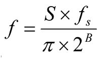Slew rate is usually specified in units of volts per microsecond (V/µs), whereas on the rate-of-change graph the vertical-axis units are the equivalent frequency in kHz—a better (ie, more general) means of expressing the same thing. If the rate-of-change graph peaks at 6kHz, for instance, then the severest rate of change within this track is equal to that of a full-scale sinewave at 6kHz. This figure is calculated by first determining the difference in sample value between adjacent samples and then converting that figure to an equivalent frequency using the equation shown at above right where S is the slew rate in LSB per sample period, fs is the sampling rate in hertz, and B is the resolution (bit depth) of the WAV file.

If nothing else, the rate-of-change findings for the DVD-As and SACDs analyzed here is of historical significance because of the flurry of interest in amplifier slew rate that occurred during the late 1970s. As readers who were audiophiles at the time will probably not need to be reminded, slew-rate limitations were offered, principally by Walter Jung [and Matti Otala—Ed.], as one of a variety of explanations for "amplifier sound."

This was a balloon that, with characteristic pragmatism, Peter Baxandall in the UK set out to burst by the simple expedient of measuring the signal rate of change actually delivered by music LPs (this was before domestic digital audio). Using a simple analog measurement technique of an RC differentiator circuit connected to an oscilloscope, Baxandall was unable to measure a slew rate higher than 0.14V/µs, equivalent under the measurement conditions to an equivalent full-scale frequency (Baxandall referred to it as a critical frequency) of about 2.2kHz. Even allowing for a safety margin, any amplifier with a power bandwidth of 20kHz or more—which any amplifier worthy of the description "hi-fi" would be expected to achieve—should cope comfortably. (Walt Jung and others factored this safety factor into their recommendations on the assumption that distortion would begin to rise long before the slew rate limit was reached, a situation that Baxandall pointed out wasn't necessarily the case.)

I'm not aware of anyone having repeated these measurements with CD, although I can't believe this was never done. The enhanced bandwidth capabilities of DVD-A and SACD offer the possibility that Baxandall's figure will be comfortably surpassed, and indeed on most of the assessed recordings it is. But even the severest examples, as you'll see, don't exceed an equivalent frequency of 12kHz. Moreover, it is clear from the DVD-A rate-of-change graphs (in the SACD ones, the signal's rate of change is largely swamped by the high level of ultrasonic quantization noise) that the average rate of change is much lower than the peak figure, so for the vast majority of the time an amplifier should be cruising in this respect. In light of these findings, it is difficult to see how an amplifier's slew-rate capability can have much to do with any sound-quality difference that is persistent rather than, at best, episodic.

Power envelope
Fourth and last of the graphs generated for each track picks up on some work I originally did in 2000 for Hi-Fi News, itself a continuation of work begun by NAD in the 1980s. This was the period when a number of manufacturers launched so-called "commutating" power amplifiers, which used switchable voltage rails to provide increased short-term power capability. (The Carver Cube, Hitachi Dynaharmony range, and NAD's PowerTracker amplifiers all fell into this general category.) These amplifiers' raison d'être was that reproducing music signals more often requires short bursts of power than the continuous power measured in conventional amplifier tests. NAD attempted to quantify this burst power requirement in the form of a "power envelope"—a plot of the required dynamic power capability vs time duration. The result of its experiments was a sigmoid (S-shaped) curve reaching a maximum value of just under 5dBr at 20 milliseconds and decreasing to zero at 3 seconds.

NAD's work was conducted before the tools became available to access directly the data in digital recordings, and so relied on the observation of oscilloscope traces—clearly a less than ideal methodology. By the time I took a belated second look at the issue, this was no longer the case: ripping a CD to hard disk for analysis was dead easy. So I wrote some software to measure the maximum RMS signal amplitude over time frames ranging from 2 milliseconds to 4096 milliseconds (4.096s), across the whole of a sound file. The latter figure may seem an odd choice, but it reflects the fact that the time frames were scaled as powers of two; ie, 2, 4, 8, 16, 32, 64, 128, 256, 512, 1024, 2048, and 4096ms.

That first piece of power-envelope analysis software was crude, to say the least; it worked with ASCII rather than binary files, and it needlessly recalculated data as a result of analyzing the file over each size of time frame in turn. To apply the same analysis to the DVD-A and SACD transfers, I rewrote the code to read WAV files directly and cut out the duplicated calculations.

Fig.4 illustrates the methodology, using the simple example of a file exactly 24ms in length. First, the RMS level in each of the twelve 2ms frames making up the file is calculated and stored. Then adjacent pairs of 2ms fames are combined to form 4ms frames, for which the RMS level is easily calculated from the 2ms frame data. Note that the 4ms frames are constructed in two ways: the first with no offset from the start of the file, the second with an offset of one of the 2ms frames. Once the RMS level of all the 4ms frames has been calculated, the highest value is stored. A similar process is then used to construct 8ms frames from four adjacent 2ms frames. This time, four 2ms frame offsets are possible: 0, 1, 2, and 3. And so on and so forth, out to the 4096ms frame length in the full analysis.

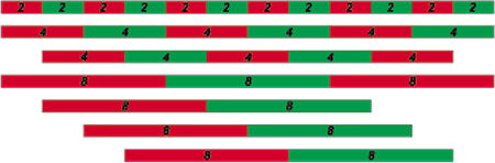
Fig.4 Example frame alignments for the power-envelope test, for frame lengths of 2-8ms. Adjacent frames in each sequence are alternately colored for clarity.

The power-envelope graphs in this article are calculated in exactly this way, which means—if you haven't already twigged—that they are less than rigorous. Because to be certain that you have captured the highest RMS signal level within each time interval, you need to repeat the above process many times, offsetting the start point by one sample each time through the initial 2ms frame. Only then will every possible time window have been assessed. For a 192kHz sound file there are 384 samples per 2ms frame, so the analysis has to be repeated with 384 different sample offsets.

If all the signal data are held in RAM, this doesn't take unfeasibly long. But if you have to rely on virtual (hard disk) memory, it takes an age. The latter was the position I found myself in (yes, you're right—oodles of RAM is high on the shopping list for my next computer), so all the power envelopes for this piece were calculated using zero sample offset only. My defense is that, based on past experience, the errors that result are relatively minor, as I hope fig.5 will persuade you.

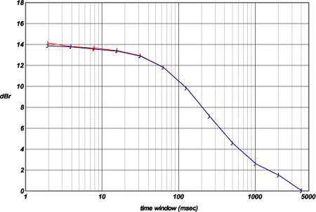
This power-envelope graph, like those that follow, has two curves—but unlike them, these do not represent the left and right channels. Rather, these results were both generated from the left channel of "Easy Does It," one of the DVD-A tracks analyzed. Here the blue plot represents the zero-offset data, as you'll find reproduced in the power-envelope graph for this track, whereas the red plot represents a full analysis, assessed over all 192 sample offsets. (This track was transferred to hard disk at 96kHz via S/PDIF, not recorded at 192kHz via the analog route, hence the reduced number of offsets—one reason I chose this track, since it halves the calculation time.) As you can see, the disparity between the two traces is, as advertised, quite small.

What do the power-envelope results mean? Let's perform an example calculation. Assumptions: speaker sensitivity 89dB, 3m (10') listening distance, uncorrelated left and right channels, no room contribution, and a volume setting such that the loudest 4096ms signal segment produces an average sound-pressure level of 100dB. The power output per channel required to achieve this is 57W. To achieve 16dB above this—about the largest 2ms dynamic power requirement identified by my measurements—means the amplifier must be able to deliver 2.27kW, albeit only over this short time span, in order to prevent clipping. You can chip away at this figure in various credible ways, but the point is made: to achieve realistic loudness levels with many types of recorded music requires substantial reserves of amplifier power—or unusually sensitive loudspeakers. No wonder it is a common reaction to hugely powerful amplifiers that they impart a sense of ease and unfettered dynamic range that lesser amps fail to emulate.

And so we come to the analysis results themselves. Before I invite you to pore over them at your leisure, I should make clear that in two cases I deliberately included notionally equivalent material (Tchaikovsky's Overture 1812 and "Easy Does It") that has been released on both DVD-A and SACD. Although this somewhat reduced the range of material that was assessed overall, I thought it would make for some interesting comparisons—which, now I've seen the outcome, I believe it does. A general note: the narrow spikes visible in the noise floor of some spectra are thought to be caused by interference from the recording/analysis computer and should be ignored.

---

Footnote: Keith Howard, for many years editor of the UK magazine Hi-Fi Answers, is currently Consultant technical editor, Hi-Fi News, Technical consultant, Autocar, Special contributor, Motor Sport, and a contributor to Racecar Engineering.