Features

By contrast, fig.17 shows the excess-phase response of the speaker whose step response was shown in fig.11. This model uses a sloped front baffle and a crossover with first-order acoustic slopes to give a time-coherent performance on the listening axis. There's a little bit of positive error at high frequencies, meaning that the microphone is just a little high of the optimal axis.

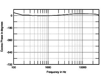
Fig.17 Acoustic excess phase response of time-acoherent loudspeaker.

But, as I said above, the fact that almost no loudspeakers perform in this manner does not stop many of them from getting good reviews, either in this magazine or in others.

Delayed Resonances
By taking a loudspeaker's impulse response, applying a window to the time data, using the FFT operation described in the sidebar to produce an amplitude response plot [35], then repeatedly moving the window along in time by an arbitrary number of samples and again taking an FFT, a three-dimensional graph can be produced [36]. This Cumulative Spectral-Decay (CSD) or "waterfall" plot—amplitude is plotted against frequency on the x axis and against time on the z axis—can be revealing of resonant problems in a loudspeaker's acoustic output that might not be associated with a peak in the amplitude response.

As mentioned in the sidebar, the shorter the time record examined, the higher the frequency at which meaningful data starts and the larger the gap between the frequency bins in the plot. With the physical conditions in the room in which I measure loudspeakers for Stereophile, I can get a reflection-free time window of around 3.5-4ms, meaning that the lowest frequency at which meaningful data exists is (1000/3.5)Hz or (1000/4)Hz = 250-285Hz. In the graphs for Stereophile, therefore, I don't plot data below 300Hz. The resolution in these plots is sufficient to reveal woofer and midrange cone problems at the top of their passbands, as well as tweeter resonances. The FFT window chosen has an effect on the display: the shorter the window's risetime, the more true the CSD plot is to the loudspeaker's transient behavior; however, by choosing a longer risetime, frequency-domain aspects are more easily seen.

Fig.18, for example, shows such a plot calculated for a small two-way loudspeaker, with the data windowed to exclude both the time of flight and any reflections from room boundaries and microphone stand hardware that might have been present. The FFT window was a Blackman-Harris type with a risetime of 0.15ms. The first dome resonance from the metal-diaphragm tweeter can be seen as a ridge of delayed energy at 27kHz. A second, less severe resonance-induced ridge can be seen at 3kHz, associated with a small peak in the amplitude response. It dies away relatively quickly, but its presence will make this speaker somewhat intolerant of recordings that have a little too much energy in the same region. (Some listeners might call this character "analytical.")

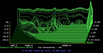
Fig.18 Typical cumulative spectral-decay plot (0.15ms risetime).