Reference

Results
The test procedure was as follows: an FFT-derived spectral analysis was performed on the processor's clock jitter (the LIMD output) when the processor was driven by the digital code representing a 1kHz sinewave at six input levels ranging from 0dBFS to -90dBFS. The FFT plots show energy vs frequency. The spectral analysis was repeated with the processor under test driven by digital silence (all data words are zero), a 1kHz squarewave, and a 10kHz sinewave at 0dBFS (full scale). The LIMD output was then connected to a true-RMS voltmeter and the jitter voltage measured with all the signals described above. The processors were all driven from the same transport (a JVC XLZ-1010) via the same digital interconnect (footnote 7). Because it would be impossible to publish nine plots for each product, I've selected the most interesting from each, usually the worst performance. If two graphs are printed, they are the usually the best and worst from the processor.

Before looking at the tested processors' jitter, let's acquaint ourselves with what to look for in these plots and see how the jitter is correlated with the audio signal.

Fig.7 is the Forté F 50 DAC's jitter spectrum when driven by the code representing a full-scale, 1kHz sinewave. Though the level is extremely low—20ps—note the spike at 1kHz and multiples of 1kHz—2kHz, 3kHz, 5kHz, 7kHz, 11kHz—indicating that the DAC's word clock is being jittered at 1kHz—the same frequency as the test signal. Now look what happens when we drive the same processor with the code representing full-scale sinewaves of 4kHz (fig.8) and 10kHz (fig.9). These plots clearly demonstrate that the jitter is correlated with the analog signal represented by the digital code—the music. Moreover, the jitter present at the DAC's word clock is also influenced by the input signal level. Fig.10 shows the Forté F 50 DAC's spectrum when driven by the code representing a 1kHz, -70dBFS signal. Note how the jitter's spectral distribution varies as a function of input level.

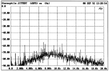
Fig.7 Jitter Spectrum, Forté F50 DAC processing 1kHz sinewave at 0dBFS (linear frequency scale, 0dB = 226.8ns, 1% of the 44.1kHz word spacing of 22.7µs). Note strong components at 1kHz—the signal represented by the data!—and its harmonics.

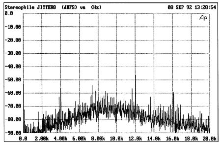
Fig.8 Jitter Spectrum, Forté F50 DAC processing 4kHz sinewave at 0dBFS (linear frequency scale, 0dB = 226.8ns). Note strong components at 4kHz, 12kHz, and 8kHz.

Fig.9 Jitter Spectrum, Forté F50 DAC processing 10kHz sinewave at 0dBFS (linear frequency scale, 0dB = 226.8ns). Note strong component at 10kHz.

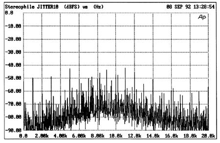
Fig.10 Jitter Spectrum, Forté F50 DAC processing 4kHz sinewave at -70dBFS (linear frequency scale, 0dB = 226.8ns).

To best assess the various aspects of each processor's jitter performance, I've organized the data gathered (over 130 FFTs and a similar number of voltage measurements) into Table 1. The following information is presented:

• Jitter level in picoseconds, best case;

• Jitter level in picoseconds, worst case;

• Number of spectral spikes that rise 10dB or more above the overall level, best case;

• Number of spectral spikes that rise 10dB or more above the overall level, worst case;

• Average level of three highest spikes, best case; and

• Average level of three highest spikes, worst case.

The "best" and "worst" cases refer to each processor's best and worst performance, which varied with the input signal level. In each of these measurements, the lower the numbers the better the performance. (Keep in mind that 1000ps equals one nanosecond.)

The average level of the three highest spikes is an expression of the peak-to-average ratio—how high the spikes rise above the average level, expressed in dB. Remember, the spikes indicate that the jitter has a specific frequency, a condition more sonically degrading than jitter with a random frequency distribution. It isn't just the jitter level that matters, but how much of the jitter energy is concentrated at specific frequencies. Note that the spikes contribute very little to the RMS level. It should also be recognized that processors with very high levels of clock jitter but no spikes on the FFT may still suffer from periodic jitter; the spikes could be buried beneath the very high average level.

Table 1

Product	Jitter (ps) Best	Jitter (ps) Worst	Spikes +10dB Best	Spikes +10dB Worst	Highest 3 Spikes Best (dB)	Highest 3 Spikes Worst (dB)	Input Receiver
Bitwise Zero	1971	2819	3	23	21	23	Yamaha YM3623B
CAL Sigma	425	440	9	17	23	27	Crystal CS8412C
EAD DSP-7000t*	168	210	8	26	16	21	Crystal CS8412C
Forté F50	20.1	25.3	10	40	14	28	Philips SAA7274
JVC XLZ1010	51	713	1	43	14	37	None
Levinson No.30	218	384	7	43	16	32	Custom
Meitner IDAT	78	82	0	0	4	5	Custom
PS UltraLink	139	177	11	41	18	28	Yamaha YM3623B
Sumo Theorem	1248	25,920	6	51	21	27	Yamaha YM3623B
Theta Gen.III	172	378	1	3	9	17	Crystal CS84l2C
Vimak DS-2000	34.8	34.9	10	22	19	20	Crystal CS8412B
VTL Reference	540	992	1	24	12	20	Yamaha YM3623B

*in 8x-oversampling mode

It was fascinating to look at the clock jitter present in digital processors with whose sound I was intimately familiar. As I saw patterns emerging between the processors' musical characteristics and their jitter performance, I began to predict the jitter level and spectrum just before attaching the probe to the DAC's word clock. So strong was the correlation between certain aspects of the processors' sonic presentation and jitter characteristics that my predictions often came close to their measured performances.

Generally, processors with none or only a few discrete frequency spikes—like the CAL Sigma shown in fig.11—are missing low-level detail, but don't sound metallic and hard in the treble. They can also sound smooth but somewhat uninvolving. Processors with a large number of discrete jitter components—the Forté F 50 DAC seen in fig.10—tend to sound forward and etched, and present brittle textures. Those rare processors with low jitter levels and absences of periodic jitter tend to sound the best. These are overly broad generalizations—there are many more factors that influence sound quality than jitter—but an overall trend was nevertheless suggested by the measurements and auditioning.

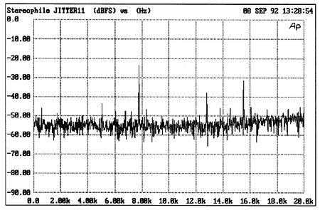
Fig.11 Jitter Spectrum, CAL Sigma processing 1kHz sinewave at -20dBFS (linear frequency scale, 0dB = 226.8ns). Jitter mainly random noise, with only a few discrete components.

The California Audio Labs Sigma, reviewed in October 1992, had a reasonable level of jitter (425ps, fig.11) and was also relatively free of discrete-frequency jitter components, particularly at lower levels. This corresponds to my general model of the correlation between jitter type and sound quality: the Sigma had a smooth treble, soft bass, and a loss of low-level detail. Conversely, the Forté (also reviewed in October 1992), with many discrete-frequency jitter components, tended to be aggressive, analytical, and brittle in the mids and treble.

The Meitner IDAT (to be reviewed next month) had very low jitter (78-82ps) and exhibited a complete absence of LIM and interface-induced discrete-frequency jitter components (fig.12). This is not surprising in light of the fact that the IDAT was designed with the aid of the LIMD, an advantage not previously available to designers of the other processors tested. The IDAT uses a custom input receiver and features two stages of Museatex's C-Lock clock-jitter reduction circuit, one of them just before the DAC. The IDAT was also unique in that the jitter spectrum was virtually identical regardless of input-signal frequency or amplitude. (It should be noted that, at its 8x sampling frequency, this level of jitter is near the LIMD's noise floor.)

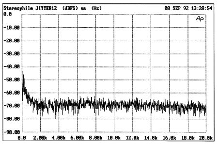
Fig.12 Jitter Spectrum, Meitner IDAT processing 1kHz sinewave at 0dBFS (linear frequency scale, 0dB = 226.8ns). Jitter very low in level and almsot completly random in nature.

The Theta DS Pro Generation III was also very good, with a low overall jitter level (172-378ps) and few discrete components. Like many of the processors tested, the Gen.III was much better behaved at high input levels. Fig.13 is the Gen.III's worst performance, with an input level of -90dBFS.

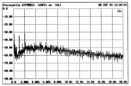
Fig.13 Jitter Spectrum, Theta DSPro Gen.III processing 1kHz sinewave at -70dBFS (linear frequency scale, 0dB = 226.8ns). Jitter very low in level, with just two data-related components (these still very low).

Although the Mark Levinson No.30 (reviewed in February '92) had low jitter (218-384ps), these figures were higher than expected considering the No.30's custom input receiver and superb sound quality. At full scale, the No.30 had very few spikes, but showed an increasing number of periodic jitter components as the input level decreased. Compare the No.30's spectrum at full scale (fig.14) and at -90dB (fig.15). Because it wasn't practical to get inside the temperature-controlled towers that house the DACs, I measured the No.30's jitter at the pin of the chip driving the ribbon cable that connects the DAC board to the main board. If the No.30 does have a reclocking circuit next to the DAC (the best place for it), the processor's actual jitter performance could be much better than that presented here. The No.30's clock signal is balanced but it was only possible to measure one half of the signal. This will also make the No.30 look worse.

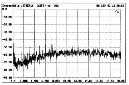
Fig.14 Jitter Spectrum, Mark Levinson No.30 processing 1kHz sinewave at 0dBFS (linear frequency scale, 0dB = 226.8ns). Jitter very low in level, with a few discrete components. Note absence of data-related 1kHz component.

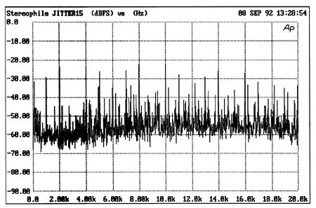
Fig.15 Jitter Spectrum, Mark Levinson No.30 processing 1kHz sinewave at -90dBFS (linear frequency scale, 0dB = 226.8ns). Many more data-related jitter components compared with fig.14, but overall level still quite low.

---

Footnote 7: The Audio Precision System One's digital signal generator had so much jitter that it significantly skewed the results, necessitating using a CD transport and test disc.—Robert Harley