| Columns Retired Columns & Blogs |
Fried R/4 loudspeaker Measurements
Sidebar 2: Measurements
The impedance plot of the Fried R/4 (fig.1) shows a single well-damped resonant peak at 50Hz, and an impedance magnitude which stays well above 5 ohms at any frequency. The speaker should be an easy load to drive. The small tick in the magnitude plot at just under 200Hz likely indicates a serious resonance somewhere in the system, something which the results below might shed some light on. The impulse response in fig.2 shows a clean decay with no serious aberrations or ringing, though the step response (fig.3) reveals that the midrange response lags the tweeter by a fraction of a millisecond—a common result. It also shows that while the tweeter and midrange unit are connected in positive acoustic polarity, the woofer is connected in negative polarity and lags the midrange unit's output.
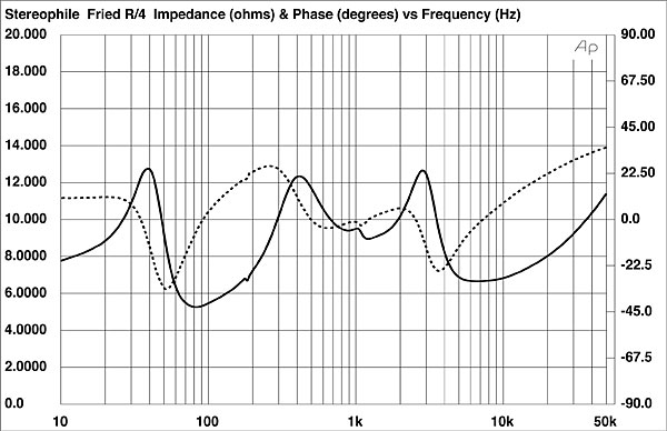
Fig.1 Fried R/4, electrical impedance (solid) and phase (dashed) (2 ohms/vertical div.).
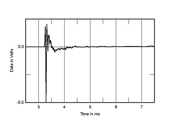
Fig.2 Fried R/4, impulse response on tweeter axis at 45" (5ms time window, 30kHz bandwidth).
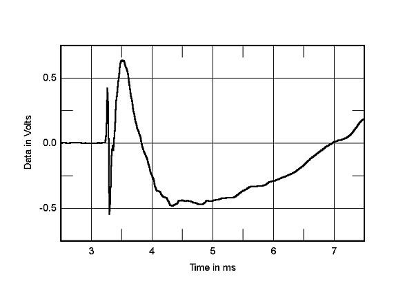
Fig.3 Fried R/4, step response on tweeter axis at 45" (5ms time window, 30kHz bandwidth).
The averaged frequency response of the R/4 across a 30° lateral window centered on the midrange axis is shown in fig.4. The shows a very smooth response in the midrange and treble. There's nothing here to explain the sometime brightness I noted in my listening tests, though the treble does rise a little above 8kHz on the tweeter axis. As plotted, there appears to be a rise in the bottom end which was not reflected in the listening tests. But remember that the level matching between the left-hand, nearfield curves and the right-hand quasi-anechoic trace in this kind of graph has to be arbitrary. Had the woofer and tunnel outputs been calculated a little lower in level, then there would appear to be a depression between 80Hz and 500Hz which would correlate with my feeling of a somewhat lean balance in this region.
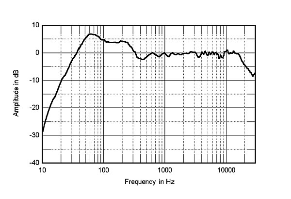
Fig.4 Fried R/4, anechoic response on tweeter axis at 45", averaged across 30° horizontal window and corrected for microphone response, with complex sum of nearfield woofer and line tunnel responses plotted below 200Hz.
Note two characteristics of red curve in fig.5—taken nearfield at the line-tunnel output. The first is the fact that the line-tunnel is apparently tuned to the same frequency as the woofer itself (blue trace), which would appear to be consistent with the design objectives (the tunnel does not operate as a reflex duct). The second is the strong resonance at about 200Hz, close to the same point at which we observed a wrinkle in the impedance plot. This resonance may also relate to the slight aberrations I noted in the lower range of some male vocals. The fact that the problem was not audibly severe indicates that it is fairly well down in level relative to the woofer's output in the same region. But the fact that it is within a few dB of the line-tunnel's bass output would also seem to indicate that the latter's contribution to the system's bass output level is not a major factor.
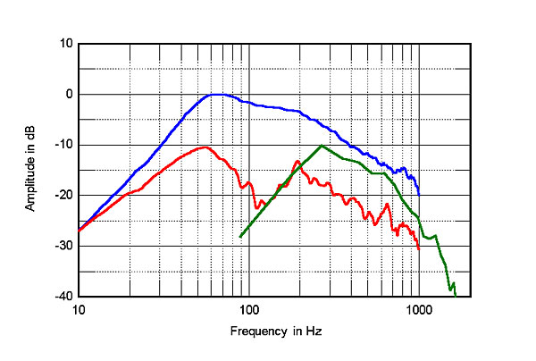
Fig.5 Fried R/4, nearfield woofer (blue), line tunnel (red), and rear port (blue) responses.
That is not to say that it doesn't make an important contribution to the system's overall bass character due to its loading effect on the woofer and enclosure, merely that its output level is not comparable with that of the woofer. That certainly puts the system closer in function to that of a closed box than that of a ported one; in the latter, the port takes over a major portion of the output function below the frequency at which the woofer itself starts to roll off.
The green trace in fig.5 shows the nearfield response of the output of the rear port, which is the opening of the open line behind the midrange driver. Since there's no way to clearly relate its absolute level to that of the front radiation, I must depend on my listening tests to tell me whether or not it might be a factor in the system's overall sound. Those tests tell me that it probably was not, but that if the system is used close to a rear wall, potential problems from the reflection of this radiation off of the nearby wall surface might result. Not a certainty, but something to keep in mind if your situation requires such a placement.
The horizontal response family, normalized to an idealized, flat on-axis response, shown at the top, is shown in fig.6. It is by no means certain that the broad rises in the lower treble and upper midrange off-axis response below and above 3kHz were responsible for the problems noted in the R/4's sound, but they fall in regions which would correlate with this. The vertical response family in fig.7 indicates that the correct vertical listening axis is fairly critical with the R/4—good reason why the system was designed with its distinctive back-tilt. Interference dips between the midrange and tweeter are quite noticeable as you move further away from the optimum vertical axis in either direction.
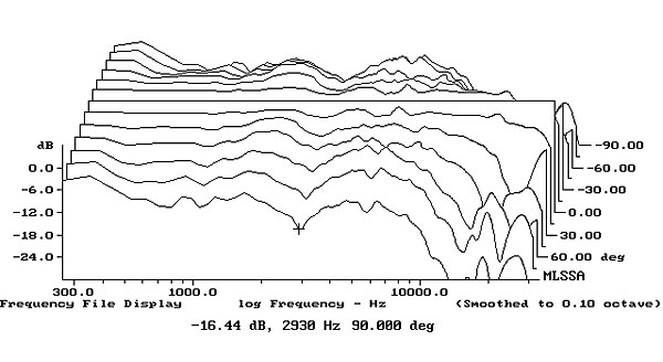
Fig.6 Fried R/4, lateral response family at 45", normalized to response on midrange axis, from back to front: differences in response 90–15° off axis, reference response, differences in response 15–90° off axis.
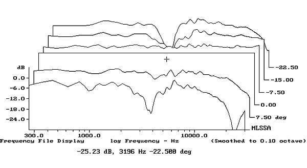
Fig.7 Fried R/4, vertical response family at 45", normalized to response on midrange axis, from back to front: differences in response 15–5° above axis, reference response, differences in response 5–10° below axis.
Fig.8, the cumulative spectral-decay or waterfall plot on the tweeter axis, shows a fairly clean result, though a series of low-level resonances can be seen between 2kHz and 8kHz. There is an on-axis rise in the top end (recall that our other plots averaged the response across a frontal, 30° window on the midrange axis), though a small portion of it is in the measurement microphone response. (The latter deviation has been equalized out of our other curves, but not the spectral-decay plots.) A nearfield response taken at the line-tunnel is shown in fig.9. It shows the previously mentioned approximately 200Hz resonance as well as another, lower-level resonance just below 100Hz.
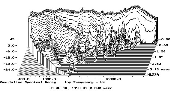
Fig.8 Fried R/4, cumulative spectral-decay plot on tweeter axis at 45" (0.15ms risetime).
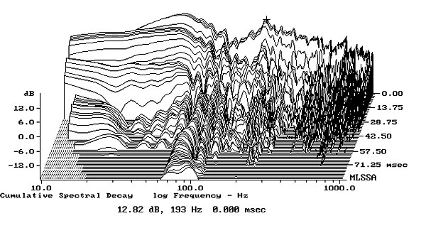
Fig.9 Fried R/4, cumulative spectral-decay plot of line-tunnel output.
A loudspeaker's enclosure itself is alive with motion on a microscopic but clearly significant level. We recently acquired an accelerometer—a device which, to simplify matters a bit, responds to vibrations in the surface to which it is attached in an analogous fashion to the way a microphone responds to vibrations in the air....The measurements were made by applying the signal from our MLSSA test set to the loudspeaker in the normal fashion, but by reading the loudspeaker enclosure's output with the accelerometer rather than measuring the system's acoustical output with a microphone. An FFT of the data was performed in the usual fashion, and a spectral-decay curve plotted out.
Readings were taken at several points on the cabinet walls; the strongest modes in the Fried R/4 plot (fig.10) fell at just under 200Hz and about 250Hz, the latter relating well with a previously noted resonance.—Thomas J. Norton
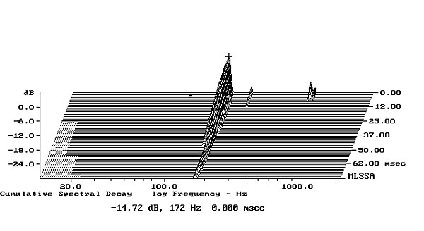
Fig.10 Fried R/4, cumulative spectral-decay plot calculated from output of accelerometer fastened near to the bottom of a side panel (MLS driving voltage to speaker, 7.55V; measurement bandwidth, 2kHz).
NEXT: Specifications »
|
|
| ||||||||||
- Log in or register to post comments


| Loudspeakers Amplification Digital Sources | Analog Sources Accessories Featured | Music Columns Retired Columns | Show Reports | Features Latest News Community | Resources Subscriptions |
 © 2024 Stereophile
AVTech Media Americas Inc., USA
All rights reserved