Stand Loudspeaker Reviews

Sidebar 3: Measurements

The SC-I is very sensitive for a relatively small speaker, its calculated B-weighted sensitivity being around 90dB/2.83V/m. However, though it will therefore play loud with low-powered amplifiers, it is a fairly demanding load, as can be seen from its plot of impedance magnitude and phase against frequency (fig.1). Though the electrical phase angle is small above the bass-enclosure resonance, the magnitude is lowish, remaining below 6 ohms over most of the audioband and dropping to a minimum value of 3.25 ohms at 260Hz. The uniformity of the curve, however, indicates that the speaker will not change its tonal balance significantly when driven by an amplifier with a high output impedance, like a classic tube design.

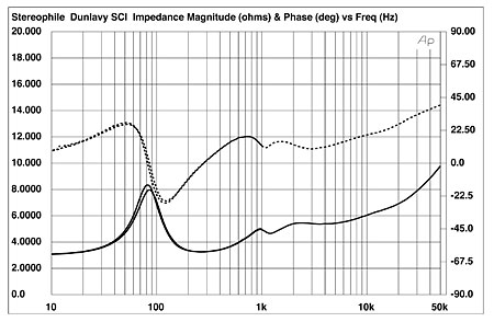
Fig.1 Dunlavy SC-I, electrical impedance (solid) and phase (dashed) (2 ohms/vertical div.). The upper trace in the bass is after 12 hours of high-level break-in with the XLO/Sheffield Lab Test CD, Track 8.

The sealed-box bass tuning is revealed by the small peak centered on 84Hz before break-in, which is high in frequency, as expected from the sensitivity. (All things being equal, the higher a speaker's sensitivity, the necessarily more restricted must be its low-frequency extension.) After break-in, this dropped slightly in frequency, to 80Hz, as revealed by the upper solid trace in fig.1. The impedance traces are free of the small wrinkles and discontinuities that would reveal the existence of cabinet or cone resonances, apart from a slight contour in the upper midrange, presumably due to an equalization network.

The use of first-order crossover filters with their shallow rolloff slopes gives rise to significant overlap between the drive-units. This can be seen in their individual response curves (fig.2), taken using DRA Labs' MLSSA system with a B&K 4006 microphone, corrected for its own departure from flatness. Though the nominal crossover frequency lies at 3.5kHz, there is a region of about an octave either side where the rolled-out driver is not that far below the selected one. This sharing of the drive signal results in an increase in the effective drive-unit size in this frequency region. This in itself is of no concern, but it does place great demands on the speaker's designer to ensure evenness of the speaker's radiation pattern off-axis.

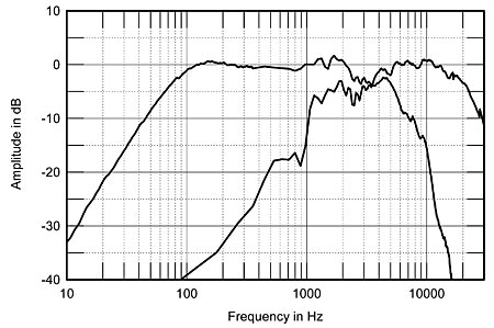
Fig.2 McCormack Micro Integrated Drive, small-signal 10kHz squarewave into 8 ohms.

The woofers can be seen to roll off quickly above 5kHz, with no apparent break-up peaks in the trace, while the highish enclosure tuning results in a low-frequency response that starts to roll out relatively early, reaching a nearfield –6dB point at 55Hz. While the slope is the gentle 12dB/octave of a sealed box, which means that the room is able to give more reinforcement to the SC-I's midbass balance than it would with a similar reflex design, the intrinsically high tuning frequency will still result in a lightweight overall balance.

I did two complete sets of on-axis system-response measurements: one at my normal distance of 50", which gives better resolution in the midrange; the other at 100", this closer to the 10' specified by Dunlavy Audio Labs. With first-order crossover filters, the degree of integration between the drivers is going to be significantly more dependent on distance than with designs using higher-order filters. John Dunlavy points out that a symmetrical array of loudspeaker drivers acts in a manner analogous to a camera with a fixed-focus lens. In the case of the SC-I's spaced twin woofers with a center tweeter, the sound will not be focused at close distances. Fig.3 shows the SC-I's response averaged across a 30° horizontal window on the tweeter axis at the greater distance. The first thing to note is the exceptionally flat response trend, with each slight peak balanced by a slight dip. Other than in the low treble, this speaker meets superb ±1.5dB limits.

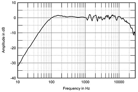
Fig.3 Dunlavy SC-I, anechoic response on tweeter axis at 100" averaged across 30° horizontal window and corrected for microphone response, with nearfield woofer response below 300Hz.

In fact, measurements made by John Dunlavy of the same samples of the SC-I in his large anechoic chamber were even better than this, the maximum deviation from flat being no more than 1dB above or below the mean. I suspect that at the 100" distance I used for this measurement, residual room reflections gave rise to the larger response ripples. In the 1–2kHz region, the peakiness became significantly worse if I removed the grille: this speaker must be auditioned with its grille in place to get the flattest on-axis balance. In any case, this is superb measured performance.

Fig.4 reveals how the SC-I's balance changes to the speaker's sides. (The on-axis response in this graph is represented by a straight line, so that just the changes off-axis can be easily seen.) The speaker maintains its fundamentally flat response across the band up to 10° off-axis. Farther than that, and a trough at 3kHz and a slight peak above it develop due to the woofers becoming more directional at the top of their passband compared with the tweeter at the bottom of its operating band. The tweeter's top-octave output also falls off a little more rapidly than usual at extreme off-axis angles, presumably due to its recessed mounting.

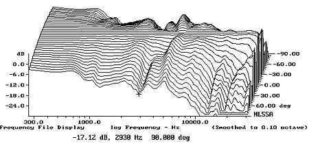
Fig.4 Dunlavy SC-I, horizontal response family at 50", normalized to response on tweeter axis, from back to front: differences in response 90°–5° off-axis; reference response; differences in response 5°–90° off-axis.

Vertically (fig.5), if you sit too high or low, a peak appears in the mid-treble, while a suckout appears in the midrange due to negative interference between the two woofers. Don't listen to this speaker standing up!

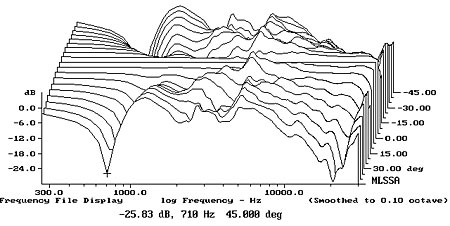
Fig.5 Dunlavy SC-I, vertical response family at 50", normalized to response on tweeter axis, from back to front: differences in response 45°–5° above reference axis; reference response; differences in response 5°–45° below reference axis.

The effect of the SC-I's vertical and horizontal dispersion behaviors will be to add a degree of brightness in live-sounding rooms, particularly if the speaker is placed close to the side walls. In my room, the Dunlavy's spatially averaged response(footnote 1, fig.6) does reveal a slight excess of mid-treble energy which is probably what I heard on uncorrelated pink noise. This is more than the Spica TC-60 which I also review in this issue, for example, but about the same as the B&W Silver Signature that I reviewed last June. More importantly, and ignoring the slight peaks and dips below 400Hz that are residual room-mode effects, the SC-I's in-room balance gently slopes down below the midrange. This relative lack of low-frequency support leads to a balance that sounds intrinsically lean, unless the speakers are moved closer to the wall behind them.

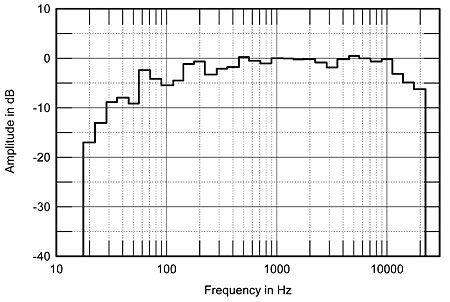
Fig.6 Dunlavy SC-I, spatially averaged 1/3-octave response in JA's listening room.

In the time domain, the SC-I's impulse response (fig.7) is indicative of a minimum-phase system. The step response (fig.8) is superb in its right-triangle shape. The ripples in the tail are due to the residual room reflections that I mentioned earlier, and should be ignored. Though the degree of overshoot on the step's leading edge is a little higher than ideal, this is due to the measuring microphone I use having a slight (1.8dB) rise on-axis in its top octave (see November '94, p.71). I allow for this in my frequency-response measurements, but its effect is present in the time-domain graphs.

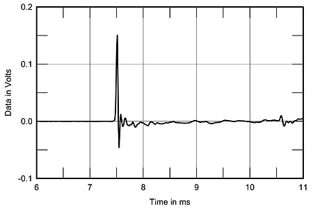
Fig.7 Dunlavy SC-I, impulse response on tweeter axis at 100" (5ms time window, 30kHz bandwidth).

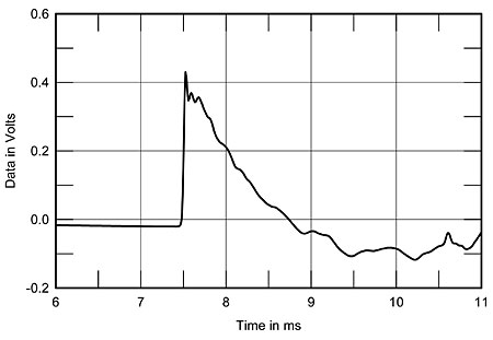
Fig.8 Dunlavy SC-I, step response on tweeter axis at 100" (5ms time window, 30kHz bandwidth).

These excellent pulse and step shapes imply that the speaker's phase response is similarly excellent. Fig.9 shows the SC-I's excess phase plotted against frequency. "Excess" phase is the speaker's actual phase response with the phase deviations associated with the speaker's departure from flat response subtracted; in the case of the Dunlavy, it varies by no more than ±5° from 400Hz to 4kHz. The slight positive phase angle, increasing with frequency in the high treble, implies that I didn't have the microphone exactly on the tweeter axis, but probably to one side. At 15° at 10kHz, however, this is negligible, implying that the tweeter's acoustic center was positioned just 1.4mm behind that of the woofers. (The wavelength of sound at 10kHz is 35mm or so.)

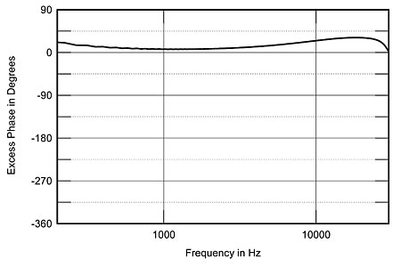
Fig.9 Dunlavy SC-I, excess phase on tweeter axis at 100" (0.025ms delay).

For comparison, fig.10 shows the excess phase curve for a typical, good-sounding three-way speaker with a flat baffle. The huge negative phase angle in the treble means that the sound from the tweeter arrives at the microphone significantly before that from the speaker's midrange unit. No way can the sounds add in-phase. There is no comparison with the SC-I. The combination of a first-order crossover and a recessed tweeter results in the outputs of the drivers all adding in-phase at the listening position to give a time-coherent performance. The SC-I joins that select group of loudspeakers capable of reproducing acoustic squarewaves with a correct square waveform.

Fig.10 Snell Type C/V, excess phase on tweeter axis at 50" (0.038ms delay).

The cumulative spectral-decay, or waterfall, plot for the SC-I (fig.11) reveals a very clean initial decay, particularly in the tweeter's passband. (Ignore the ridge at 16kHz, which is due to my computer monitor's screen.) Some apparent resonant modes develop in the upper midrange, around the cursor position at 2kHz. These may correlate with the hardness to the speaker's sound I noted at high levels.

Fig.11 Dunlavy SC-I, cumulative spectral-decay plot at 100" (0.01ms risetime).

Finally, the SC-I's cabinet walls do suffer from a couple of strong resonant modes in exactly the region I suspected when I was breaking the speakers in. Fig.12, a waterfall plot revealing the cabinet's side-wall behavior, reveals that the SC-I's small cross-sectional area—associated with increased stiffness—and the use of bracing has pushed what modes there are well up into the midrange, to 560Hz and 660Hz. Their level is relatively high, however. This will be partly because the SC-I's high sensitivity results in greater stimulation for the same electrical drive. Nevertheless, on some instruments such as flute, and on female voice, the cabinet could be heard to add a slight degree of overhang to the sound. This is presumably because the frequencies of these panel resonances coincide almost exactly with the frequencies of the notes D and E at the top of the treble staff (assuming the standard instrumental tuning based on A = 440Hz), and thus will be almost continually excited by Western music. Other designers have found that if such resonances fall in the cracks between the notes, they will have less of a subjective effect (unless the speakers' owner likes to play recordings tuned to a lower A—to the 409Hz typical of baroque music, say). I suspect that these cabinet modes do contribute to the high-level hardness I noted.—John Atkinson

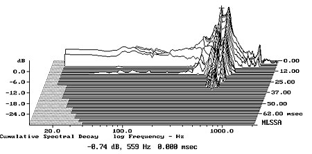
Fig.12 Dunlavy SC-I, cumulative spectral-decay plot of accelerometer output fastened to center of enclosure side panel halfway up from the base. (MLS driving voltage to speaker, 7.55V; measurement bandwidth 2kHz.)

---

Footnote 1: I average six measurements at each of 10 separate microphone positions for left and right speakers individually, giving a total of 120 original spectra, which are then averaged to give a curve which, for my room at least, has proved to give a nice correlation with a loudspeaker's perceived balance.—John Atkinson