Stand Loudspeaker Reviews

Sidebar 2: 1989 Measurements

Each speaker was submitted to the following measurement schedule: The voltage sensitivity was assessed with 1/3-octave pink noise centered on 1kHz, while the change of impedance with frequency was measured using spot tones (footnote 1). The nearfield low-frequency response of each speaker was assessed with a sinewave sweep to get an idea of the true bass extension relative to the level at 100Hz.

The frequency response of each speaker in the listening area was measured using pink noise and an AudioControl Industrial SA-3050A 1/3-octave spectrum analyzer. Nine sets of six averaged measurements were taken independently for left and right loudspeakers at a distance of just over 2m in a window 72" wide and varying from 27" to 45" high. The response shown in each review is the average of these measurements, weighted slightly toward the sound heard at the listening position. This spatial averaging is intended to minimize the effect of low-frequency room standing-wave problems (below 500Hz or so) on the measurement, and gives a response curve that has proved to predict reasonably well what is heard; it also gives an idea of the off-axis behavior of the speaker under test.

In addition, for these tests, I captured the impulse response of the speakers using a PC-compatible, 8-bit Heath/Zenith digital storage 'scope. This enables up to 250 separate "snapshots" to be averaged, which (as long as the time relationship between the trigger pulse and the captured pulse is constant, within one sampling period) usefully increases the S/N ratio. The 'scope communicates with the computer via its RS232 port, the computer then controlling the 'scope's settings via "soft" keys. The waveform can be stored on disk as a 512-point ASCII file, which thus enables the user to carry out various mathematical operations on the data. Accordingly, I wrote an FFT program in Microsoft's Quickbasic 4.5 language (footnote 2), which takes about two minutes to calculate the equivalent anechoic response of the speaker from the impulse data file (footnote 3).

The measurement window was 10ms, it being assumed that the impulse has died away to zero by this time (footnote 4), and I arranged the position of the speakers so that any reflections of the pulse from room boundaries would arrive after this period. The trigger to the 'scope was a delayed twin of the analytical pulse, the delay time approximately arranged to coincide with the transit time of the sound from speaker to measuring microphone. In addition, use of a 10ms window results in a sampling frequency of just under 51.3kHz, minimizing audio-band aliasing.

I have included these responses in the measurement sections of the reviews, but note that I have only plotted the range—from 200Hz to 10kHz—where the calculated responses have proved to be repeatable within 0.25dB or so. (To cover the entire audio spectrum, a unidirectional square pulse needs to be of no more than approximately 20µs in length; the pulse I was using, shown in fig.1, was unfortunately 55µs long, curtailing the accuracy of the measurement in the top audio octave. Note that the pulse used has inverted polarity: this is due to the inverting line stage of the Conrad-Johnson PV9 preamplifier used for these tests. A 20µs pulse generator is on the way, as is a math coprocessor chip.

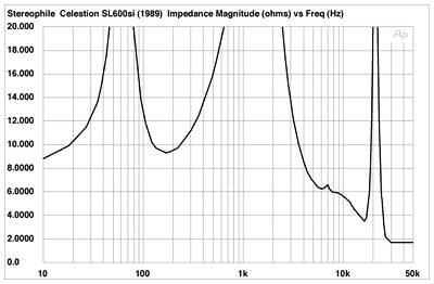
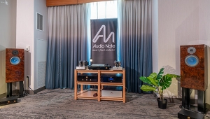
Fig.1 Celestion SL600si, electrical impedance (2 ohms/vertical div.)

Note also that a 10ms window means that you are stuck with 100Hz resolution: midrange peaks and dips due to resonances and interference that are narrower than this will be lost. On the other hand, going to a 20ms window, say, if the room were large enough and the speaker far enough above the floor, would halve the measurement bandwidth with only 512 data points. A case of swings and roundabouts, I guess.)

The 600Si's impedance plot is shown in fig.1. With enclosure and tweeter resonances lying at 60Hz and 1200Hz respectively, the value stays above 8 ohms until 4kHz or so. The entire treble is shelved down, however, presumably due to the tweeter designer trying to squeeze sufficient sensitivity from it, indicating that current-meager amplifiers are best avoided with this loudspeaker. The low 82dB/W/m sensitivity also indicates that low-power amplifiers are also to be avoided. This is one fussy loudspeaker when it comes to choosing a matching amplifier. The very sharp peak at 21kHz is due to the notch filter used to counteract the tweeter's high amplitude peak at resonance.

Measured in the nearfield, the bass extension was moderate, the -6dB point relative to the level at 100Hz lying at 47Hz. The rate of roll-off was shallow, however, resulting in an in-room response (fig.2) with useful small-signal extension to around 36Hz. The spatially averaged in-room response reveals the tweeter to be about 2.5dB too low in level referred to the mean woofer level. The latter is a little lumpy in the upper bass, and also around 600Hz or so. On-axis, the tweeter response is rising a little by 20kHz, but it is so directional at this frequency that the overall response is down a little. At the bottom of the tweeter's passband, the response is characterized by a lack of energy in the octave between 2 and 4kHz, this worsening off the speaker's direct axis and below the tweeter axis. The SL600Si is therefore a speaker that must be listened to on the correct axis if the high treble is not to become too depressed and the presence region too sucked-out. (The depression was only 3dB with the microphone level with the cabinet top.)

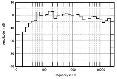
Fig.2 Celestion SL600si, spatially averaged, 1/3-octave, freefield response in JA's Santa Fe listening room.

Fig.3 shows the 600Si's response to a 55µs unidirectional rectangular pulse, taken just above the tweeter, which will correspond to the listening axis. The initial response is inverting (remember the test pulse was negative-going) due to the tweeter being connected in reverse polarity, as is usual with a symmetrical, 12dB/octave crossover. Note how, in comparison with a time-coherent design like the Vandersteen 2Ci, the bulk of the energy takes considerably longer to arrive, almost 2ms in fact, due to the non-time-coherent nature of the crossover and drive-unit placement. The ringing in the impulse tail has a frequency of around 7.5kHz; I have no idea of its cause, but it probably isn't coincidence that a small peak appears in the impedance plot (fig.1) at the same frequency.

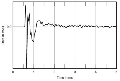
Fig.3 Celestion SL600si, impulse response on tweeter axis at 12" (5ms time window, 25kHz bandwidth).

The FFT-derived amplitude response (from a 10ms window rather than 5ms) can be seen in fig.4. Again in contrast to the Vandersteen, note how the use of second-order slopes and a reversed tweeter polarity results in an ostensibly flat amplitude response, this being achieved, however, at the expense of the time-domain performance. Which is more important depends on the designer's (and listener's) priorities—these two speakers admirably demonstrate the two extremes. For some reason, the 2-4kHz depression in the in-room response doesn't show in fig.4; this is a function of the microphone position used to capture the impulse response, reinforcing the idea that the optimal listening axis is slightly above the tweeter. Noticeable, however, in both figs.2 and 4, is the peak at 600Hz. (It also appears in the measurements of the SL600Si published in the March 1989 issue of Hi-Fi Choice.) This excess energy may correlate with the occasional feeling of slight midrange confusion or thickening noticed on audition.

Fig.4 Celestion SL600si, FFT-derived anechoic response on tweeter axis at 12".

However, it doesn't show on the plots of the individual drive-unit responses, measured in the nearfield (fig.5), which suggests that, perhaps, it is a cabinet phenomenon. Martin Colloms conducted accelerometer measurements on the original '600's back panel, which showed a vibrational mode at about 650Hz—see HFN/RR, May 1983, p.58. I remember some discussion at that time, though, which suggested that mistermination between the woofer cone and the surround at that frequency was the culprit, which is presumably why the woofers of the SL6S and SL700 use composite surrounds with two different compliances. If that is true, then I am a little puzzled as to why Celestion decided to stick with the single surround for the '600Si woofer (footnote 5).

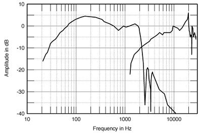
Fig.5 Celestion SL600si, acoustic crossover, measured in the nearfield.

Whatever, the SL600Si's woofer can be seen to be fairly well-behaved overall, with a steep acoustic roll-out above crossover over which is superimposed a series of dips which I suspect are more a result of interference phenomena due to the nearfield microphone placement than to actual cone breakup. (The latter was blamed for just about all the woes of the modern world by J. Peter Moncrieff in his review of the original SL600 and SL6 in IAR Hotline #35.)

Looking at the tweeter response in fig.5 (strictly speaking, this is not a nearfield measurement except in the bottom few octaves of its range, due to the small wavelengths at 10kHz and above), it can be seen that it both has a deficiency of energy immediately above crossover and is set a little too low in level. The subjective balance of the SL600Si is, I am sure, while musically pleasing, therefore a function of the limited tweeter sensitivity. Padding down the woofer might produce a flatter response overall, but the system sensitivity would then drop to the point of unacceptability. Its delayed roll-in would also explain the lack of energy in the 2-4kHz region seen in fig.2. The tweeter starts its rise toward resonance above 15kHz, this reaching +6dB by 20kHz before the notch filter cuts in.

The debate still continues (see my interview with Robin Marshall in February, Vol.12 No.2) as to whether this resonance should be notched out or allowed to ring free. From tracing out a neat peak between the shoulders either side of the notch at 20kHz and 23.4kHz, it would seem that without the filter, the tweeter resonance peak would rise at least 12dB above the drive-unit's nominal reference level, which may well lead to intermodulation problems if allowed to ring out unrestrained.—John Atkinson

---

Footnote 1: It has been worrying me for some time that while my impedance plots are the right shape, the absolute values differ slightly from the manufacturer's specification and from those published in other magazines. In particular, speakers reach a slightly higher impedance value at their LF resonance, though this itself is not changed in frequency. After considerable head-scratching, the acquisition of some even-higher-precision calibration resistors than I used before, and the purchase of a new Fluke 87 true-RMS multimeter, I can only conclude that it must be the effect of the reduced air pressure here in 7000'-high Santa Fe.

Footnote 2: To those laymen like myself who find themselves interested in FFT techniques, I found Ronald Bracewell's The Fast Fourier Transform and Its Applications (McGraw-Hill) to give a usefully thorough exposition of the theory. The appendix to Williams's and Taylor's Electronic Filter Design Handbook (Second Edition, McGraw-Hill) was also of help.

Footnote 3: So much toil to end up with the DIY equivalent of Julian Hirsch's IQS FFT analyzer! I have always believed, however, that the heuristic approach is the best way to gain an understanding of how test equipment works. You can then appreciate its limitations when faced with the real-world task of coping with the foibles of music reproduction systems.

Footnote 4: This may be an unjustified assumption. I will be trying various shaped windows, such as the Hamming, which imposes a raised cosine amplitude function on the windowed data, in future tests.

Footnote 5: I suspect they felt that this would render the sound too much unlike the traditional SL600 sound.