Stand Loudspeaker Reviews

Other than impedance, for which I use an Audio Precision System One, all acoustic measurements were made with the DRA Labs MLSSA system and a calibrated B&K 4006 microphone. I place the speaker under test on a turntable/stand so as to place its tweeter about halfway between the listening-room floor and ceiling and midway between the sidewalls. Then, on the floor between the speaker and microphone, I construct an acoustic "black hole" out of graded layers of acoustic foam and fiberglass damping material, which kills the forward floor reflections of the sound emitted by the speaker. The primary reflection in the MLSSA's calculated impulse response is, therefore, that of the tweeter from the ceiling, which arrives about 4ms after the direct sound. This 4ms reflection-free time window results in a measurement valid down to 300Hz or so. To minimize reflections from the test setup, the measuring microphone was flush-mounted inside the end of a long tube. Reflections of the speaker's sound from the mike stand and its hardware will be sufficiently delayed not to affect the measurement.

The frequency response is calculated from this impulse response using the Fast (Discrete) Fourier Transform and is corrected for the measuring microphone's on-axis departure from a flat response. I then take the impulse responses of the low-frequency driver(s) and port(s)/passive radiator(s) in the nearfield, with the tip of the microphone capsule almost touching the centers of their cones/apertures, and append these responses to the upper-frequency ones. To calculate the overall low-frequency rollout, DRA Labs' software allows you to add the complex responses (amplitude and phase) of the woofer and port or sub-bass unit in the ratio of their diameters.

Because Santa Fe's 7000' altitude reduces the sensitivity of all loudspeakers, I calculate sensitivity by comparing the measured, B-weighted level at 50" for a given voltage input, using a noise signal, with that obtained for a sample Rogers LS3/5A that I've measured both in Santa Fe and at sea level.

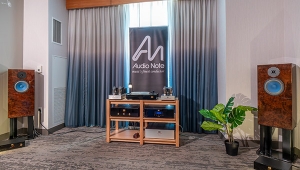
As expected from such a small enclosure, the Lynnfield 300L is not very sensitive. Specified at 83dB/W/m, its B-weighted figure was actually a little higher, at 85dB. However, its plot of impedance magnitude and phase (fig.1) revealed the speaker to be relatively easy for an amplifier to drive, only dropping below 6 ohms in the lower midrange. The tuning of the reflex port is indicated by the frequency of the impedance "saddle" between the two bass peaks, 40Hz, which suggests quite good low-frequency extension for such a small box. No wrinkles in the impedance traces can be seen, implying a relative absence from major cabinet resonances.

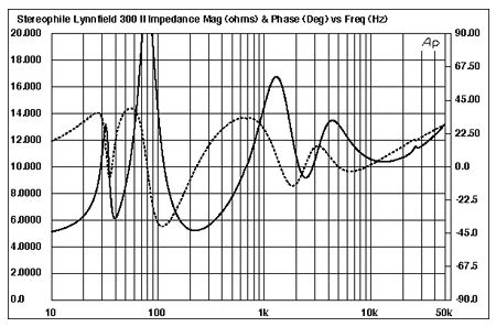
Fig.1 Boston Acoustics 300L, electrical impedance (solid) and phase (dashed) (2 ohms/vertical div.).

Fig.2 shows the individual responses of the tweeter, woofer, and port. The latter is the sharp-peaked bandpass trace, centered on 38Hz or so. The port appears to have a reasonably severe resonant peak around 700Hz. The woofer itself starts to roll out below 120Hz, suggesting that the 300L's designer has chosen quite a high-Q bass alignment to stretch downward what would otherwise be a somewhat lightweight balance. The tradeoff that this produces, as I found in my auditioning, is a rather indistinct bass character possessing a modicum of weight but lacking definition.

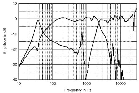
Fig.2 Boston Acoustics 300L, acoustic crossover on tweeter axis at 50", corrected for microphone response, with nearfield woofer and port responses plotted below 300Hz.

Higher in frequency, the woofer is basically flat on-axis throughout the midrange, overlaid by a slight rising trend, then rolling off steeply above 2kHz. A couple of resonant peaks can be seen above its passband, but these are well-suppressed by the high-order crossover. The tweeter is also basically flat in its passband, with a sharp notch at the tweeter resonant frequency of 26.5kHz that I assume is due to the Amplitude Modulation Device in front of the dome.

Fig.3 shows the Lynnfield 300L Series II's overall frequency response on the tweeter axis, averaged across a 30° horizontal window to smooth out inconsequential, position-dependent anomalies. Other than a slight peak at the reflex tuning frequency—correlating with the uneven bass definition I noted—the bass is shelved down. This, taken with the slight rising trend throughout the midrange to the mid-treble, will render the speaker's tonal balance a little bright. The treble, however, is basically flat on-axis, so there should not be any emphasis of sibilants—as, indeed, I found.

Fig.3 Boston Acoustics 300L, anechoic response on tweeter axis at 50", averaged across 30° horizontal window and corrected for microphone response, with complex sum of nearfield woofer and port responses plotted below 300Hz.

For reference, fig.4 shows the response of the first version of the Lynnfield 300L. Very similar in the bass—David Fokos told me that it wasn't possible to change the woofer's parameters—it otherwise tilts up with frequency to a much more significant degree than the Series II speaker. Note that I was much bothered by this aspect of the earlier 300L's tonal balance. The balance of the revised Lynnfield is much improved, in my opinion.

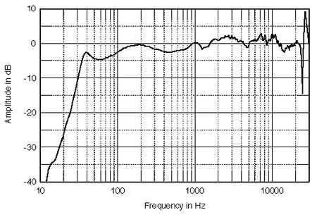
Fig.4 Boston Acoustics 300L, Series I, anechoic response on tweeter axis at 50", averaged across 30° horizontal window and corrected for microphone response, with complex sum of nearfield woofer and port responses plotted below 300Hz.

Contrary to popular belief, brightness is not associated with too much high-treble energy but with excesses lower down in frequency—I would not have expected the 300L's slight energy excess through the top of the midrange to the mid-treble in the on-axis response to make the sound over-bright. Still, with prolonged listening, this aspect of the speaker's balance annoyed me more and more. The plot showing how the 300L's response changes to its sides (fig.5) suggested a second possible reason: the speaker has a very wide lateral dispersion at the bottom of the tweeter's passband, but is more beamy above and below that region. Not by a large amount—the small-diameter woofer will inherently have quite a wide dispersion above 1kHz—but enough to accentuate the on-axis balance's tendency to brightness.

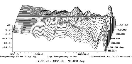
Fig.5 Boston Acoustics 300L, horizontal response family at 50", normalized to response on tweeter axis, from back to front: differences in response 90°–5° off-axis; reference response; differences in response 5°–90° off-axis.

The 1/3-octave plot of the 300L's in-room balance (fig.6) confirms this hypothesis. Assessed at the listening position in my room, the low- and mid-treble are shelved up by 2–3dB compared with the midrange, which will make the balance a little bright. ( For my in-room spectral analyses I average six measurements at each of 10 separate microphone positions for left and right speakers individually, giving a total of 120 original spectra. These are then averaged to give a curve that, in my room, has proved to give a good correlation with a loudspeaker's perceived balance. I use an Audio Control Industrial SA-3050A spectrum analyzer with its own microphone, which acts as a check on the MLSSA measurements made with the B&K mike. I also used the Goldline DSP-30 automated spectrum analyzer.)

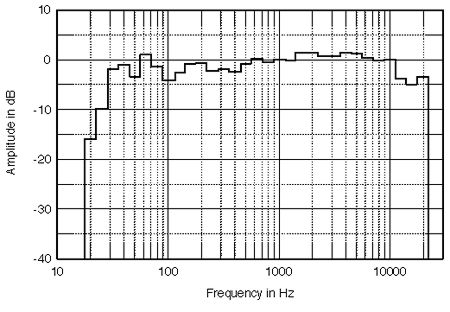
Fig.6 Boston Acoustics 300L, spatially averaged, 1/3-octave response in JA's room.

Vertically (fig.7), the 300L is quite fussy when it comes to choosing the optimal listening axis. Move more than 5° above the tweeter and a suckout appears in the crossover region. Things are less critical below the tweeter axis, however, so make sure you sit on or just below the tweeter to be sure of getting the best midrange/treble transition.

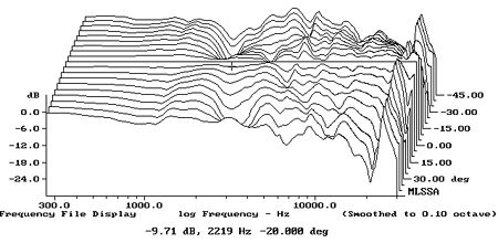
Fig.7 Boston Acoustics 300L, vertical response family at 50", normalized to response on tweeter axis, from back to front: differences in response 45°–5° above tweeter axis; reference response; differences in response 5°–45° below tweeter axis.

In the time domain, the 300L's step response (fig.8) holds no surprises, the two drive-units being connected in the same (positive) acoustic polarity, but with the tweeter's output leading the woofer's by about 0.3ms. The associated cumulative spectral-decay or waterfall plot (fig.9) reveals a basically clean decay but with a few residual modes present in the mid-treble, presumably due to the woofer's cone breakup behavior. Note the suppression of a ridge of resonant energy at the tweeter's ultrasonic resonance frequency; the AMD appears to do its job.

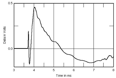
Fig.8 Boston Acoustics 300L, step response on tweeter axis at 50" (5ms time window, 30kHz bandwidth).

Fig.9 Boston Acoustics 300L, cumulative spectral-decay plot at 50" (0.15ms risetime).

Finally, I used a simple plastic-tape accelerometer to investigate the cabinet's resonant behavior. For my cabinet resonance tests, the speaker is placed on upturned cones (which allow all the various modes to develop to their fullest) and excited with a 2kHz bandwidth MLS signal at a level of 7.55V RMS. (See Stereophile, June 1992, p.205; and September 1992, p.162.)

Fig.10 shows a waterfall plot calculated from the accelerometer's output when it was fastened to the front baffle just above the tweeter. Though a ridge of delayed resonant energy can be seen at the cursor position (250Hz), this is well down in level. There are a couple of modes apparent higher in frequency in this plot; the one at 500Hz could also be found on the 300L enclosure's side and top panels, but was strongest on the AMD bar in front of the woofer! The subjective effect of this behavior is unpredictable, though I do wonder if it ties in with the hardness to the speaker's sound I noted at high levels.—John Atkinson

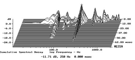
Fig.10 Boston Acoustics 300L, cumulative spectral-decay plot of accelerometer output fastened to front baffle above tweeter (MLS driving voltage to speaker, 7.55V; measurement bandwidth, 2kHz).