| Columns Retired Columns & Blogs |
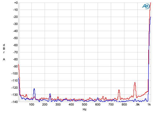
The -112dBW unweighted residue noise is spectacular.
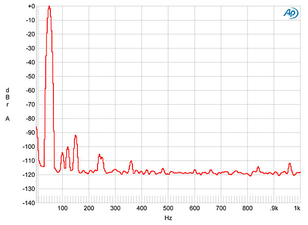
However, in figure 4, the 120Hz hum noise component is only -100dB below the 2.83V signal. Is it something going on?
I performed a full set of measurements using my Audio Precision SYS2722 system (see www.ap.com and the January 2008 "As We See It"). Before taking any measurements, I preconditioned the Ayre by running it for 60 minutes at one-third the specified power into 8 ohms, which is very much the worst case for an amplifier with a class-B or class-A/B output stage. Like the original MX-R, the MX-R Twenty got hot, the temperature of its heatsink fins reaching 140.3°F (60.2°C) and the top of its case 116.1°F (46.8°C). The THD+noise measured 0.03% with the amplifier cold, and stabilized at 0.0178% with the amplifier hot. While the Ayre's unusual heatsink has sufficient thermal conductivity to be effective for an amplifier of this power rating, the MX-R does need to be used in a well-ventilated space.
The voltage gain into 8 ohms was a little lower than the specified 26dB, at 25.1dB, and the amplifier preserved absolute polarity, its XLR jack being wired with pin 2 hot. The input impedance is specified at a very high 2 megohms. Though it is difficult to measure an impedance this high with any accuracy, my measurement indicated that the input impedance was at least 1M ohm across the audioband. Like the original MX-R, the output impedance was higher than usual for a solid-state design: 0.26 ohm at low and middle frequencies, rising to 0.28 ohm at 20kHz, with a slight dependence on the load impedance. (Both the value of the impedance and the dependence are due to the absence of overall loop negative feedback.)
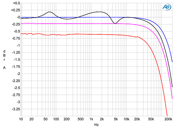
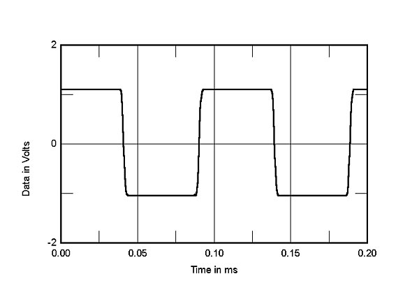
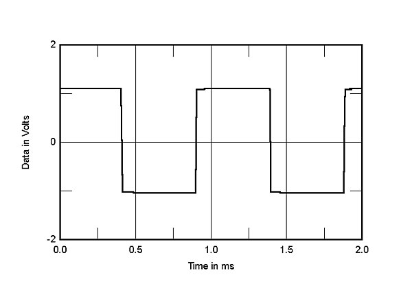
This higher-than-usual output impedance results in a slight (±0.24dB) variation in frequency response with our standard simulated loudspeaker (fig.1, gray trace). The MX-R Twenty, however, offers a very wide small-signal bandwidth, especially into higher impedances. Into 8 ohms (fig.1, blue trace), for example, the upper –3dB point is above 200kHz, the limit of this graph, and at 200kHz the response is down by just 1.5dB. This wide bandwidth correlates with the excellent shape of a 10kHz squarewave (fig.2), with very short risetimes and no overshoot or ringing. A 1kHz squarewave was reproduced with an essentially perfect shape (fig.3).
The original MX-R was a quiet amplifier, but the Twenty handily exceeded it. With the amplifier's input shorted to ground, the unweighted, wideband signal/noise ratio (ref.1W into 8 ohms) measured an extraordinarily low 109.9dB, this improving to 112.1dB when the measurement bandwidth was restricted to the audioband, and to 113dB when A-weighted. The blue trace in fig.4 shows a low-frequency spectral analysis of the MX-R Twenty's output while it drove a 1kHz tone into 8 ohms. The individual random noise components all lie close to –140dB, and while power-supply–related spuriae can be seen at 120 and 240Hz, these lie at a superbly low –121 and –129dB, respectively. The red trace in fig.4 shows what happens when the output power is increased to 100W into 8 ohms. Supply-related sidebands now appear at ±120 and ±240Hz, but these are still at or below –112dB (0.0025%).
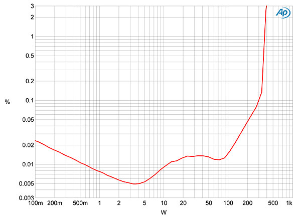
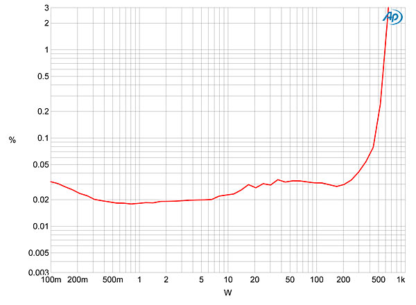
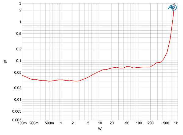
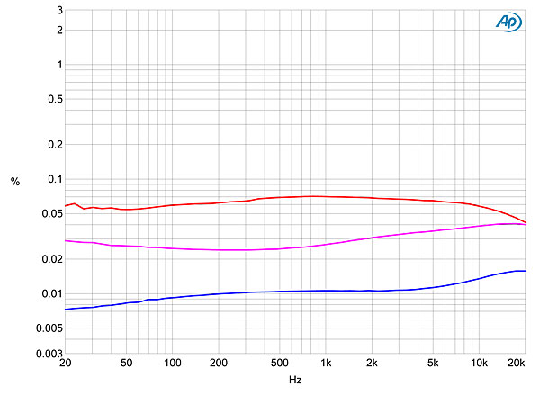
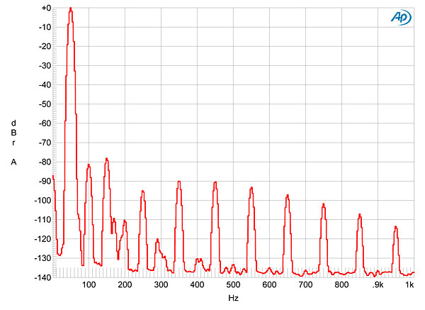
Figs. 5–7 respectively plot how the percentage of THD+N in the Ayre's output changes into 8, 4, and 2 ohms. With our definition of clipping as being when the THD+N reaches 1%, the MX-R Twenty comfortably exceeds its specified power of 300W into 8 ohms (24.8dBW). With the wall voltage at 122.4V AC, the Ayre clipped at 360W into this load (25.6dBW) and the distortion remained below 0.02% below 100W. Into 4 ohms the amplifier clipped at 595W (24.7dBW), and into 2 ohms it clipped at 720W (22.55dBW), though the distortion was higher at lower powers into these loads. (The wall voltage was 119.7V at the clipping point into 2 ohms.) This can also be seen in fig.8, which plots the THD+N percentage against frequency at 8.975V, which is equivalent to 10W into 8 ohms, 20W into 4 ohms, and 40W into 2 ohms. However, the increase in distortion into lower impedances was not as great as it had been with the original MX-R.
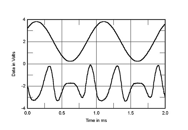
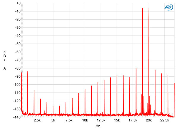
At low powers, the distortion was primarily the third harmonic (figs. 9 and 10), but at high powers this was joined by both the second harmonic, at almost the same level (fig.11), and by a regular series of higher-order products. These were associated with low-level crossover distortion that was visible on the oscilloscope screen. The original MX-R had been better behaved in both this respect and when it came to high-frequency intermodulation at high powers. While the second-order difference component at 1kHz resulting from an equal mix of 19 and 20kHz tones lay at a low –84dB (0.006%, fig.12), some higher-order products were visible, though it is fair to note that almost all of these lie at or below –90dB (0.003%).
The Twenty version of the MX-R is significantly quieter than its predecessor while offering a slightly different distortion signature. But it still packs a great deal of power into its relatively tiny frame. It is a true high-resolution amplifier.—John Atkinson
|
|
| ||||||||||

The -112dBW unweighted residue noise is spectacular.
However, in figure 4, the 120Hz hum noise component is only -100dB below the 2.83V signal. Is it something going on?

The -112dBW unweighted residue noise is spectacular.
One of the best I have measured.
However, in figure 4, the 120Hz hum noise component is only [100dB] below the 2.83V signal. Is it something going on?
The apparently anomalous behavior stems from the fact that I measure S/N ratio with the amplifier's input shorted. There is therefore no signal current being drawn from the power supply. But in my spectral analyses of the low-frequency noisefloor, I use a more realistic condition, which is with the amplifier delivering at minimum 1W into 8 ohms. In this condition, the AC transformer is being asked to deliver greater current, and the 120Hz and 240Hz spuriae appear. But at -100dB, these are still negligible.
John Atkinson
Editor, Stereophile
John:
You can't measure S/N with the inputs shorted otherwise where would you apply the signal? I believe what you meant to say is that you measured the amplifier noise floor with the inputs shorted. This makes more sense and is the correct way to do so.
You can't measure S/N with the inputs shorted otherwise where would you apply the signal? I believe what you meant to say is that you measured the amplifier noise floor with the inputs shorted.
The Signal/Noise Ratio is the measured level of the component's self-generated noise within a specified bandwidth referred to a specified level, in this case 2.83V into 8 ohms. The noise level is conventionally measured with the component's input shorted to ground.
The individual components of the noisefloor, examined in a separate measurement, are, of course, lower than the measured noise power used to calculate the S/N ratio, as the latter is the RMS sum of those components.
The poster's argument was that if spectral analysis showed that a supply component at 120Hz was present at -100dB ref. 2.83V, the unweighted RMS sum of the noisefloor components used to calculate the S/N ratio couldn't be less than 100dB.
John Atkinson
Editor, Stereophile
So the left/right channel inputs are shorted together and both fed a 2.83V mono signal? Sorry being dense as I'm still confused where you apply the 2.83V level signal to perform these measurements. Thanks...
So the left/right channel inputs are shorted together and both fed a 2.83V mono signal?
No, this has nothing to do with connecting the left and right inputs together. (And this is a mono amplifier, please note.) The 2.83V is the reference level at the amplifier's output. It is equivalent to a power of 1W into 8 ohms. (Strictly speaking, it should be 2.82843V, but 2.83V is close enough for this kind of measurement.)
Sorry being dense as I'm still confused where you apply the 2.83V level signal to perform these measurements.
This the procedure I use to measure S/N ratio:
Feed the amplifier an input signal at 1kHz so that the output level is exactly 2.83V RMS into 8 ohms.
Set this as the analyzer's reference level.
Turn off the signal generator. With the Audio Precision system I use, this connects both the hot and cold phases of its balanced output to ground.
Read on the analyzer's screen what the level now is, in dB referred to the previous level of 2.83V. This is the S/N ratio for whatever analyzer bandwidth I have chosen. (The Audio Precision gives me the choice of flat response from <10Hz to >500kHz or from 22Hz to 22kHz, plus the option of applying a weighting filter, like CCIR or A-weighting.)
I hope this explanation clears thing up.
John Atkinson
Editor, Stereophile
OK...thanks. That makes sense now. I wasn't aware that you ground the AP analyzer outputs after determining the reference AP voltage needed to produce a 1W amplifier output into an 8 ohm load. So the AP takes that reference signal level and divides it by the measured output noise when the amps inputs are grounded to calculate the S/N ratio. Is that about right?
So the AP takes that reference signal level and divides it by the measured output noise when the amps inputs are grounded to calculate the S/N ratio. Is that about right?
That's correct. The AP can display the noise level in dB vs an arbitrary reference, as in this case, as dBm, dBV, and other decibel-related ratios, or as the absolute level in milli- or microvolts.
John Atkinson
Editor, Stereophile


| Loudspeakers Amplification Digital Sources | Analog Sources Accessories Featured | Music Columns Retired Columns | Show Reports | Features Latest News Community | Resources Subscriptions |
 © 2024 Stereophile