| Columns Retired Columns & Blogs |
Under Pressure: Loudspeakers at Altitude Further Experiments (previously unpublished)
Postscript: Further Experiments (previously unpublished)
A 1991 trip to Atlanta and Washington DC gave me the opportunity to measure loudspeaker systems both in Santa Fe and at sea level. I took along with me the magazine's MLSSA system, mounted in a Compaq 286 transportable computer, EAR microphone preamplifier, DPA 4006 microphone, and a pair of small loudspeakers, these Wharfedale Diamond IVs on loan for review. (The review appeared in the July 1991 issue of Stereophile.) I would have liked to take a pair of panel speakers with me also, but it wasn't logistically possible to take more than one pair of loudspeakers—there is a limit to how much the airlines let you take! As the Diamond is a ported design, however, I felt it would enable me to look at differences in low-frequency behavior.
As near as I could reasonably assess, the test conditions for the measurements were identical in Santa Fe and in Washington DC—same microphone the same distance away on the same axis, the same microphone preamplifier, same cable (6' of multistrand cable), same temperature (22°C), same drive voltage measured at the loudspeaker terminals, and the same series resistor (nominal value 1000 ohms, measured value 997 ohms) to measure impedance. Although the driving amplifiers in the two sites were different, they were both Mark Levinson No.23.5s, and in the case of the impedance measurements, I measured the amplifier transfer function in each location. I can only roughly estimate relative humidity: in Santa Fe, it measured as 50%; in DC, it must have been nearer 80%, as it had been raining that afternoon.
One final difference was that the microphone to floor distance in Santa Fe was 60"; the lack of a suitable stand in DC meant that I couldn't raise the speaker so that the tweeter axis was no higher than 45" from the floor. This will give slightly different time windows before the first boundary reflection in the two situations, the Santa Fe measurement figures being accurate down to a slightly lower midrange frequency as a result.
So. What did I find?
Fig.4 Wharfedale Diamond IV in Washington DC, impedance magnitude (solid) and electrical phase angle (dotted) (2 ohms/vertical div.).
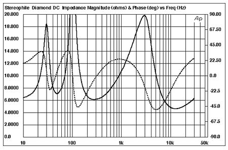
Fig.5 Wharfedale Diamond IV in Santa Fe, impedance magnitude (solid) and electrical phase angle (dotted) (2 ohms/vertical div.).

Looking at impedance first, figs.4 & 5 show the impedance magnitude and phase in Washington DC and Santa Fe, respectively. As can be seen, while there do not appear to be any significant differences above 250Hz or so, the bass tuning has been affected slightly by the reduction in air density. For convenience, I have tabulated these differences below:
Table 1: Wharfedale Diamond IV, Impedance Differences
| Feature | In Washington DC | In Santa Fe |
| Low bass peak | 18.4 ohms 29.8Hz | 18.3 ohms 31.25Hz |
| Port tuning | 7.03 ohms 48.8Hz | 7.1 ohms 46.9Hz |
| Upper bass peak | 30.5 ohms 102.0Hz | 30.9 ohms 96.7Hz |
| Upper bass minimum | 6.1 ohms 251.0Hz | 6.04 ohms 246.6Hz |
| Treble peak | 19.9 ohms 2.919kHz | 19.8 ohms 2.919kHz |
| Treble minimum | 4.69 ohms 14.404kHz | 4.63 ohms 14.815kHz |
Some prefer such minima and maxima to be quoted at the 0° phase angle point. Instead, I have quoted the actual minimum and maximum magnitudes as I have found these to be more repeatable than phase angle with FFT-based MLSSA measurements. The magnitude is quoted to the second calculated decimal place, but I would imagine that experimental error makes just the first significant. Likewise with the frequency: although I have printed what the MLSSA software gave me, I imagine three (at the most) figures only would be significant. (Repeating the measurements gives agreement only to 1Hz in the bass region, for example.)
The minimal change in port tuning frequency is, I expect, due to the reduced mass of the slug of air in the port being compensated for by the reduced compliance of the enclosed air. I would appreciate hearing from readers what they feel the other changes to be due to.
How important are these changes subjectively? The change in woofer alignment can be given a context by looking at the other Wharfedale Diamond of the pair, which was measured in Santa Fe only. (The data are given in Table 2.) Note that the upper bass peak of the second sample is higher in frequency than that of the other sample, being closer to that of the first sample measured in Washington DC. Note also that while the shape of the second sample's impedance magnitude curve is generally similar to that of the first, it differs significantly in detail, to a far greater extent than the supposed differences due to altitude as measured on the first sample. (Perfect pair matching is obviously not available at the $300/pair price point!) Yet listening to these speakers individually reveals only relatively minor differences in bass quality on music program. Subjectively, they are obviously two samples of the same design.
Table 2: Wharfedale Diamond IV, Samples 1 & 2 Impedance
| Feature | Sample 2 | Sample 1 |
| Low bass peak | 17.4 ohms 30.8Hz | 18.3 ohms 31.25Hz |
| Port tuning | 9.1 ohms 61.0Hz | 7.1 ohms 46.9Hz |
| Upper bass peak | 22.8 ohms 100.1Hz | 30.9 ohms 96.7Hz |
| Upper bass minimum | 6.19 ohms 266.1Hz | 6.04 ohms 246.6Hz |
| Treble peak | 20.0 ohms 2.963kHz | 19.8 ohms 2.919kHz |
| Treble minimum | 4.87 ohms 13.194kHz | 4.63 ohms 14.815kHz |
Okay, how about sensitivity? I captured the waveform of a 2.828V RMS, 1/3-octave wide warble tone, centered on 1kHz (Track 20 on the Stereophile Test CD) with the tip of the microphone at a distance of 1m away on the tweeter axis. The MLSSA software has a "Calculate SPL" function, which can be invoked provided the relevant microphone sensitivity and preamplifier gain has been entered. Using DPA's supplied sensitivity figure of 10.4mV/Pa and the measured preamp gain of 37.1dB, this gave a result of 82.0dBdB(B) in DC but 79.5dB(B) in Santa Fe.
The 2.5dB reduction in sensitivity in Santa Fe is significantly greater than I expected, given my calculations in the May 1990 "As We See It," which indicated an approximate 0.9dB reduction for a conventional moving-coil unit. I have no explanation for the discrepancy, unless I got my powers and pressures confused. There might have been an experimental error of some kind, of course, or the microphone sensitivity might also have dropped. (The mike's specified sensitivity was at 1014mbar—the spec. quotes a static pressure coefficient of –0.002dB/mbar at 250Hz, which you would think would be irrelevant.) There is one other possibility, which is that this is not an anechoic measurement, and the different room acoustics in the two measurement sites might have introduced an interfering factor.
Finally, the frequency domain. I took the impulse response of the Diamond with the microphone tip 1m away on the tweeter axis in both geographic locations, with both a 30kHz bandwidth and a 5kHz bandwidth. I then placed the microphone about 2mm away from the center of the woofer dustcap and about 5mm away from the center of the port and took the respective nearfield impulse responses with a 1kHz bandwidth. (The voltage drive levels were the same in both locations, of course.)
Each impulse response was transformed into a frequency response. Looking at fig.6, the black trace shows the speaker's "signature" in Washington DC, which is a composite of: the complex sum of the nearfield port output and the nearfield woofer output, plotted up to 350Hz with 2Hz resolution; and the anechoic (FFT-derived response) at 1m, plotted from 350Hz to 20kHz with 88Hz resolution. (The level-matching between each of the nearfield measurements and the anechoic measurements, of course, can only be approximate.) The red trace is the woofer's nearfield response; the blue trace is the port's nearfield response. Both graphs are normalized to 0dB at 1kHz.
Fig.6 Wharfedale Diamond IV, response on HF axis at 1m in Washington DC, with the complex sum of the nearfield LF responses with the nearfield woofer output (red) and port output (blue).

Fig.7 is the identical composite for the same loudspeaker measured in Santa Fe. Fig.8 shows the difference between the two farfield responses (Level-SF–Level-DC).
Fig.7 Wharfedale Diamond IV, response on HF axis at 1m in Santa Fe, with the complex sum of the nearfield LF responses with the nearfield woofer output (red) and port output (blue).
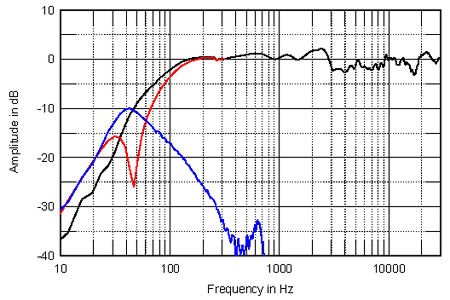
Fig.8 Wharfedale Diamond IV, difference in the speaker's sea-level response due to 7000' altitude.

To examine these graphs in detail: on a macroscopic scale the speaker's response above the upper bass region is identical in both Santa Fe and DC, with the same response step apparent between 2 and 3kHz, and the same shelved-down mid-treble. Though the difference plot appears to indicate slight changes, I have to say that these mainly are less than the differences I have measured between two nominally identical loudspeakers, as well as lying within what I regard as the experimental error due to the inability to position the microphone at precisely the same point in space.
The exception is probably the slight rising trend noted in Santa Fe compared with DC for the tweeter's response in the top two octaves plotted, which, referenced to the level at 8kHz, reaches +1.45dB at 20kHz and a maximum of +2dB at 28kHz. This would appear to indicate that the Diamond will sound very slightly more "airy" or "open" at Santa Fe's altitude than it does in sea level. (This kind of spectral tilt is not heard as "brightness.")
In the bass region, as are to be expected from the impedance measurements, there are again slight differences. The Santa Fe Diamond has a slightly more damped low-frequency alignment (the opposite of what I would have expected, perhaps due to the reduction in mass of the air slug in the reflex port), with the port output slightly suppressed in level. It might be expected that the Diamond's bass would be sound fractionally looser and very slightly deeper at sea level than in Santa Fe. But again, I must say that these differences are of the order of those between nominally identical loudspeakers, in my experience.
Nearly a decade after I performed the experiments with the Wharfedale Diamond, Stereophile relocated from Santa Fe to Manhattan. As I still had my 1978 pair of Rogers LS3/5as, which I had measured at regular intervals during my stay in the High Desert of New Mexico, one of the first things I did after I had settled in my new Brooklyn home was to perform a complete set of measurements on these speakers.
Fig.9 Rogers LS3/5a in Santa Fe, impedance magnitude (solid) and electrical phase angle (dotted) (5 ohms/vertical div.).

Fig.10 Rogers LS3/5a in Brooklyn, impedance magnitude (solid) and electrical phase angle (dotted) (5 ohms/vertical div.).

Fig.9 shows the impedance magnitude and phase of one of the LS3/5as measured in 1990 in Santa Fe at its 7000' altitude. For comparison, fig.10 shows the same loudspeaker's impedance magnitude and phase measured in 2005 in Brooklyn—altitude just 20' above sea level. As with the Wharfedale, the specific differences are given in a table:
Table 3: Rogers LS3/5a, Impedance Differences
| Feature | In Brooklyn | In Santa Fe |
| Bass peak | 59.51 ohms 90.27Hz | 57.88 ohms 81.16Hz |
| Upper bass minimum | 8.18 ohms 171Hz | 8.33 ohms 171Hz |
| Midrange peak | 35.33 ohms 786.5Hz | 35.51 ohms 786.5Hz |
| Low Treble Minimum | 12.5 ohms 1657Hz | 12.645 ohms 1657Hz |
| Treble peak | 20.1 ohms 2724Hz | 20.42 ohms 2724Hz |
| Treble minimum | 9.64 ohms 10.491kHz | 9.41 ohms 10.125kHz |
The traces in these graphs look identical, but as the table shows, there are some small differences. However, the only important difference concerns the position of the low-frequency impedance magnitude peak, which has shifted down by 9Hz at the higher altitude. Unless something physical had changed in the 15 years that separate these measurements, the speaker had more bass extension in Santa Fe, which I must admit was not something I had expected from my auditioning. This is the opposite of what had happened with the reflex-loaded Wharfedale.
Turning to sensitivity, again I used MLSSA's "Calculate SPL" function, and used the same figures for microphone sensitivity and preamplifier gain. However, for both the Santa Fe and Brooklyn measurements, I used a 20kHz-bandwidth noise stimulus. This gave a result of 83.2dB(B) in Brooklyn compared with 82.34dB(B) in Santa Fe. The reduction in sensitivity, due to the reduction in air density, appears to be 0.84dB, which is within the margin of error of the 0.9dB figure, calculated back in 1990. This makes it likely that the 2.5dB difference I noted between the Wharfedale Diamond's sensitivity in Santa Fe compared with Washington DC had been influenced by some other factor.
The frequency responses of the LS3/5a in Santa Fe and Brooklyn are shown in fig.11, with again a composite trace—nearfield below 300Hz, farfield above 300Hz—shown for each location. The responses were taken on the tweeter axis but this time each measurement was taken at a distance of 50", with the speaker raised high from the floor on a high stand to allow me to eliminate the influence of the floor reflection on the measurement.
Fig.11 Rogers LS3/5a, response on HF axis at 50" in Brooklyn (blue) and in Santa Fe (red), with the nearfield woofer responses plotted below 300Hz.
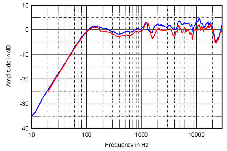
As with the Wharfedale Diamond IV, at first glance the responses look identical. Again, this is very obviously the same loudspeaker. The woofer at altitude is a little higher in level, however, as predicted by the impedance plots. While the difference in voltage sensitivity is apparent, this difference does look to be greater in the mid-treble than it does in the midrange, meaning that the LS3/5a will sound very slightly brighter at sea-level than it does at altitude. In contrast and again as with the Diamond, the speaker's top octave is balanced relatively a little higher at 7000' than it is at sea level, which might add a little extra "air" to the Santa Fe presentation. In addition, the upper-midrange peak, the height of which differs considerably between different samples of the LS3/5a, looks as if it is slightly more developed at altitude.
The difference between the LS3/5a's farfield response at sea level and at 7000' altitude is shown in fig.12; it shows the effect of the reduction in air density on the sea-level response. Unlike the similar graph for the Wharfedale (fig.8), it is hard to see an overall trend. Though there is a dB less mid-treble energy compared with the midrange, the difference in the speaker's top-octave output features as many cuts as boosts and it hard to see the apparent increase in output seen in fig.11.
Fig.12 Rogers LS3/5a, difference in the speaker's sea-level response due to 7000' altitude.

Overall Conclusion
I was reminded of this 1990 "As We See It" and the subsequent unpublished data when I read an October 11, 2005 comment on rec.audio.high-end concerning the Rocky Mountain Audio Fest. This Show took place in mile-high Colorado. The poster, one "Bear," wrote that "speakers are all designed to work properly at sea level atmospheric pressures—at the altitude that Denver is at (ca 5000' up) the air is too thin, so the 'center design point' is shifted up at least one octave. The effect is to make everything either sound like Mini Mouse (apologies to Mickey and Disney) and/or cause the bass to lack the 'weight' that it needs (again due to the gossamer lightness of the thinner air molecules)."
From my own experience, described in this report, if there is a real change in a loudspeaker's behavior or tonal balance due to the altitude at which it is used, it looks as if it is mostly swamped by the inevitable experimental error involved in measuring a speaker in different locations a decade apart. It is also similar in degree to the inevitable differences between nominally identical samples of the same loudspeaker. The only exceptions to this are the speaker's voltage sensitivity, which drops with reducing air density as expected; its top-octave output, which is tilted-up very slightly; a slight reduction in upper-bass boom with reflex designs; and a slight increase in bass extension with both sealed-box and vented enclosures.
But as for the thinner air making speakers "sound like Minnie Mouse"? No. That's just another urban legend.
Future work involves performing a full set of sea-level measurements on my B&W Silver Signature speakers, which I had also fully characterized in Santa Fe in the 1990s. I welcome feedback on this subject. Email me at the magazine's "Letters" address.—John Atkinson
|
| |||||||||
- Log in or register to post comments


| Loudspeakers Amplification Digital Sources | Analog Sources Accessories Featured | Music Columns Retired Columns | Show Reports | Features Latest News Community | Resources Subscriptions |
 © 2024 Stereophile
AVTech Media Americas Inc., USA
All rights reserved