Features

If the signal appears not to be random, then a good way to visualize its underlying structure is to plot a graph of the autocorrelation coefficient vs time lag, as illustrated in fig.3. The first graph (a) shows the autocorrelation vs lag graph for pseudo-random noise. As with any signal, the autocorrelation coefficient is 1 at lag zero because the signal is exactly aligned with itself. At lags of 1 sample and greater, the coefficient falls to within a narrow band around zero, confirming that the signal is unstructured; ie, random. Compare this with the second graph (b), which shows the result for a sinewave signal. In this case, the autocorrelation plot traces out a sine-like wave—actually a sine with a triangular envelope. Graph (c) shows what happens when the noise and sine signals are mixed: even though the RMS amplitude of the sinewave is in this case about 9dB less than that of the noise, the autocorrelation plot still reveals its presence.

Fig.3 Autocorrelation plots for (a) random noise, (b) a sinewave, and (c) a combination of the two.

On the KISS (Keep It Simple, Stupid) principle, I decided to use the lag 1 test as a measure of randomness in the quantization error signals extracted from my 24-bit files. To do this, the quantization error data was sliced up into frames 8192 samples in length (corresponding to 0.085 second at 96kHz sampling rate) and the lag 1 autocorrelation coefficient calculated for each frame. If a frame failed this test, its position was noted and autocorrelation data then calculated for lags of 0 to 4095 samples, to allow an autocorrelation plot to be generated. I wrote a little software utility to do this, and pointed it at the left and right channels of the 10 tracks listed in Table 1. Except for the last track, all of these are 24/96 recordings obtained, as already described, via S/PDIF transfer. The last and shortest track is an excerpt from one of JA's recordings, which he sent me as a 24/88.2k AIFF file. With one exception (the Ray Brown Trio's "Easy Does It"), all are digital recordings, so tape noise is not a factor.

Table 1: Music Examples Used for Analysis

Track ref.	Artist(s)	Track	Album	Label & Catalog Number
1	Dave's True Story	"Daddy-O"	Sex Without Bodies	Chesky CHDVD174
2	Sara K	"Brick House"	Hobo	Chesky CHDVD177
3	John Basile Quartet	"Desmond Blue"	The Desmond Project	Chesky CHDVD178
4	Latin Jazz Trio	"Doña Olga"	Latin Jazz Trio	AIX Records AIX 80011
5	Zephyr	"Now Is the Month of Maying"	Voices Unbound	AIX Records AIX 80012
6	Peppino D'Agostino	"Desert Flower"	Acoustic Guitar	AIX Records AIX 80013
7	Pro Arte Trio	Haydn: Piano Trio 1, Menuetto	Haydn Piano Trios	AIX Records 1340 AX
8	George Enescu Quintet	Scarlatti: Six Sonatas, No.2	Scarlatti/Beethoven	AIX Records 1341 AX
9	The Ray Brown Trio	"Easy Does It"	Soular Energy	Hi-Res Music HRM 2011
10	Robert Silverman	excerpt	Beethoven: Diabelli Variations	Stereophile STPH017-2

The results of the analysis are shown in Table 2, where the track reference numbers correspond with those in Table 1. In all but one case—which I'll return to—the number of frames failing the lag 1 test is a very small fraction of the total number of frames in the track. In two cases (one of them JA's excerpt) there are no failed frames whatsoever; in the others there are rarely more than a handful. Just as significant is how these frames are distributed within the track. Let's take the right channel of the AIX Haydn piano-trio recording as an example, which has 11 failed frames. Here the first two failed frames are contiguous and fall very early in the track, before the music starts, as the gain is being raised. The next two occur at about 112 and 190 seconds into the track, respectively, where the signal falls to a low level between sections of the music. The remaining seven failed frames all occur close to the track's end, in two blocks of three and four contiguous frames, as the gain is being faded down.

Table 2: Frame Analysis of Music Examples in Table 1

Track ref.	Channel	Failed frames
1	left	1/2355
	right	1/2355
2	left	4/4241
	right	3/4241
3	left	1/2959
	right	1/2956
4	left	1182/5339
	right	797/5339
5	left	5/984
	right	6/984
6	left	9/2762
	right	13/2762
7	left	15/3383
	right	11/3383
8	left	0/3637
	right	0/3637
9	left	1/2800
	right	2/2800
10	left	0/315
	right	0/315

If we look at the autocorrelation plot for each of these 11 frames (fig.4), we can form some idea of how audible each glitch is within the extracted quantization error signal. In the first two and last seven failed frames the glitches are very audible, and this is generally reflected in clearly structured autocorrelation plots. The remaining two frames have autocorrelation plots that look innocuous, and the corresponding glitches in the quantization error signal do indeed have to be listened for quite closely. Note that when I talk here of the glitch being audible, this is within the extracted and amplified quantization error signal. I have also listened for them within the truncated 16-bit file, and there they are very difficult to detect.

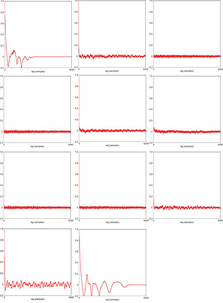
Fig.4 Autocorrelation plots for the 11 frames that failed the lag 1 test in the right channel of the Haydn piano-trio recording (Track ref. 7). Some show very obvious structure, others resemble that of random noise.

Although these autocorrelation findings broadly confirm the results of listening to the quantization error and add some rigor to the process, as I've already stated, I find the former the more sensitive and relevant test. Just occasionally, a glitch that was audible in the quantization-error files escaped detection by the autocorrelation test, perhaps because the human ear can "hear into" noise more effectively that the autocorrelation test can see into it, although I have also found the lag 1 test to be poor at recognizing the correlated quantization error generated by low-frequency sinewave signals—an effect I'm puzzling over as I write. Whatever, I'm quite sure that an elaborated test, perhaps incorporating spectral analysis, could be devised that would ensure that every nonrandom section of quantization error could be detected automatically.

This begs the question of what to do about failed frames. If there are few of them and they mostly fall, as with the Haydn example, right at the beginning or end of a track, they might safely be ignored. Or what I term a "contingent dither" solution might be applied, where dither is added only for those frames where it is required (probably being ramped up and down on either side rather than switched on and off). In a smart realization of this approach, techniques might be borrowed from perceptual coding to shape the dither such that it is masked, as effectively as possible, by the signal. The brute-force solution, of course, is to apply dither to the entire signal regardless, but if the unnecessary addition of dither is audible—as I contend—then clearly this is suboptimal.

The one track that manifestly did not fit the pattern was the Latin Jazz Trio's "Doña Olga." Here the number of failed frames was a significant fraction of the total, and a distorted version of the music could be clearly heard within the quantization error. What makes this recording different? I would guess that it's a simple matter of the microphones being subjected to higher SPLs (I'm presuming this is a "stage" rather than an "audience" mix, in AIX terminology), which results in a lower level of mike noise within the recording. Certainly the inherent noise here is lower than in the Sara K. track, as shown in fig.5. The difference in noise level appears to be about 10dB, which is sufficient to reduce it below the amplitude needed to provide effective dither at 16-bit resolution.

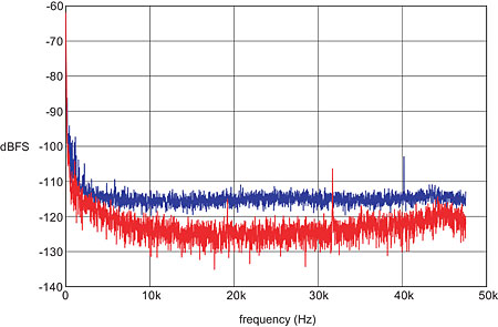
Fig.5 Noise spectrum from the beginning of the Latin Jazz Quartet's "Doña Olga" (red trace) compared with that from Sara K.'s "Brick House" (blue). The noise level in the former is about 10dB lower. (Sampling rate 96kHz and 8192-point FFT in both cases.)

Whatever you may think of my dither contentions, these results at least suggest that a significant number of 24-bit purist recordings actually don't better 16-bit performance in respect to signal/noise ratio. There are microphones available that have significantly lower self-noise than the typical 15dBA SPL I've quoted and so might alleviate this problem (the Rode NT1-A, which claims to be the world's quietest studio condenser microphone, has a noise specification of just 5dBA SPL), but recording engineers find themselves between two stools. Quieter microphones generally have larger capsules (the NT1-A's is 1" in diameter) and poor response extension above 20kHz; smaller-diameter microphones have a more extended HF response but are noisier. So a compromise has to be struck between exploiting the bandwidth and noise potentials of high-resolution recording.