Floor Loudspeaker Reviews

The quasi-anechoic measurements were all performed using DRA Labs' MLSSA system and a calibrated DPA 4006 microphone. The Aerial Acoustics 20T V2 is specified as having a voltage sensitivity of 90dB/2.83V/m; my estimate was somewhat lower, at 88dB(B)/2.83V/m on the tweeter axis, which is slightly lower than my measurement of the original 20T. The electrical impedance (fig.1), however, is very similar, with minimum values of 3.25 ohms at 24Hz and 3 ohms at 228Hz. Fortunately, the electrical phase angle at those frequencies is low, but with an impedance that stays between 4 and 6 ohms throughout most of the bass and midrange, the Aerial needs a partnering amplifier that's comfortable with driving low impedances. The impedance remains above 10 ohms in the treble, which will result in a slightly tipped-up tonal balance if the speaker is driven by a tube amplifier with a typically high output impedance.

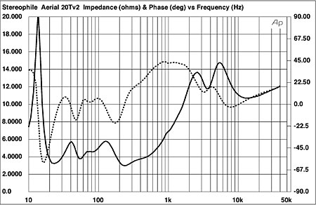
Fig.1 Aerial Acoustics 20T V2, electrical impedance (solid) and phase (dashed). (5 ohms/vertical div.)

The impedance traces are free from the small wrinkles that would indicate the existence of cabinet panel resonances. Testing with an accelerometer revealed that both the 20T V2's head unit and bass bin are extremely inert. Fig.2, for example, is a cumulative spectral-decay plot calculated from the accelerometer's output when it was fastened to the center of the head unit's sidewall. A couple of very-low-level modes can be seen around 400Hz, as well as a longer-lasting but still low-level one in the midbass.

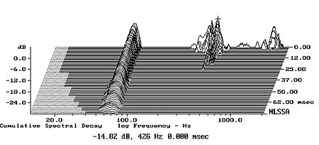
Fig.2 Aerial Acoustics 20T V2, cumulative spectral-decay plot calculated from output of accelerometer fastened to center of head-unit side panel (MLS driving voltage to speaker, 7.55V; measurement bandwidth, 2kHz).

The saddle centered at 22Hz between the two lower-frequency impedance peaks in fig.1 suggests that this is the tuning frequency of the big, downward-firing port. The red trace in fig.3 shows the port's output measured in the nearfield. It does peak between 20 and 30Hz, but there is a secondary peak an octave above the actual tuning frequency. Other than a couple of very-low-level peaks around 200Hz, the rolloff above that region is smooth. The green trace in fig.3 shows the response of the twin woofers. They behave identically, with a sharply defined minimum-motion notch at 27Hz and a steep, well-controlled rolloff above 250Hz or so. The peak in the midbass is almost entirely an artifact of the nearfield measurement technique, the tuning of the woofers being apparently maximally flat. The crossover to the midrange unit (blue trace) appears to be set at around 280Hz, and the midrange driver's rolloff is both less steep than the woofers' and broken by a small, well-suppressed peak at 80Hz, presumably the unit's tuning frequency.

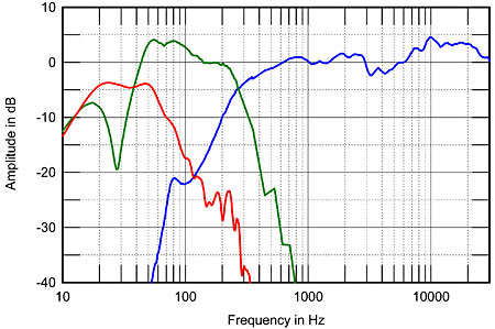
Fig.3 Aerial Acoustics 20T V2, acoustic crossover on tweeter axis at 50", corrected for microphone response, with nearfield responses of midrange unit (blue), woofers (green), and port (red) plotted below 350Hz, 800Hz, and 320Hz, respectively.

Higher in frequency in fig.3, the farfield midrange response is impressively even, though there is a shallow depression at the base of the tweeter's passband and a slight plateau in the top two octaves. (The tweeter control was set to its maximum for this measurement.) The mid-treble depression, right where the ear is most sensitive, will explain the discrepancy between my estimate of the Aerial's voltage sensitivity and the specified figure, which, I suspect, was taken on a slightly different axis (see fig.7).

To the left of fig.4 is shown the complex sum of the nearfield port, woofers, and midrange responses. Again, the midbass peak will be mostly due to the nearfield measurement technique, but it does suggest that the Aerial 20T V2 will sound bass-heavy in small rooms. The plot above 300Hz in this graph is the farfield response on the tweeter axis, averaged across a 30° horizontal angle. Though the slight depression at the base of the tweeter's passband is still evident, as is the slight top-octave plateau, the response is otherwise superbly flat and even. Fig.5 shows the effect on this response of the treble switch when set to its Boost and Cut positions. The region covered by the tweeter is increased or reduced by 1.5dB—rather a lot, considering how wide a region is covered.

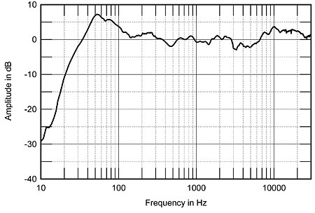
Fig.4 Aerial Acoustics 20T V2, anechoic response on tweeter axis at 50", averaged across 30° horizontal window and corrected for microphone response, with complex sum of nearfield responses plotted below 300Hz.

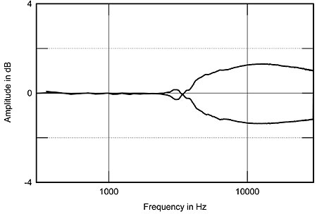
Fig.5 Aerial Acoustics 20T V2, effect of tweeter-level switch set to maximum and minimum positions, referenced to tweeter-axis response (2dB/vertical div.).

Fig.6 shows the Aerial's lateral dispersion, normalized, like the traces in fig.5, to the speaker's tweeter-axis response. Other than a small notch developing off-axis at the top of the midrange unit's passband, the radiation pattern is superbly even and well controlled. This is especially true in the region covered by the ribbon tweeter, which explains the fussiness Michael Kelly encountered when optimizing the 20T V2s' positions in my room. It looks from fig.6 as if the slight depression in the mid-treble does tend to fill in somewhat to the speaker's sides. In the vertical plane (fig.7), as hinted earlier, the depression also fills in below the tweeter axis, though the fact that the ribbon is very directional at high frequencies in the vertical plane means that you can't sit lower than the midrange unit's axis, which is 35.5" from the floor when the speaker stands on its spiked feet. Perhaps not coincidentally, my listening chair puts my ears exactly on the optimal axis. A deep suckout centered at 3.5kHz develops 5° above the tweeter axis, which suggests that this is the upper crossover frequency.

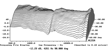
Fig.6 Aerial Acoustics 20T V2, lateral response family at 50", normalized to response on tweeter axis, from back to front: differences in response 90–5° off axis, reference response, differences in response 5–90° off axis.

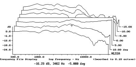
Fig.7 Aerial Acoustics 20T V2, vertical response family at 50", normalized to response on tweeter axis, from back to front: differences in response 15–5° above axis, reference response, differences in response 5–15° below axis.

The red trace in fig.8 shows the Aerials' spatially averaged response after the speaker positions had been optimized, while the blue trace is the response with the speakers as originally set up. (I perform this measurement by averaging 20 1/6-octave smoothed responses taken for each speaker individually in a rectangular grid measuring 36" by 18" and centered on the positions of my ears in my listening chair. I used an Earthworks omni microphone and a Metric Halo ULN-2 FireWire audio interface, in conjunction with SMUGSoftware's Fuzzmeasure 2.0 running on my Apple laptop.) The traces are very similar in the midrange and treble, as might be expected because the speakers' power response in these regions is not significantly affected by the changes in position. But closer examination reveals that the new placements have resulted in slightly more upper-frequency energy overall. And not revealed in this graph is that the individual responses that were averaged to produce the traces varied much less with the revised speaker positions. Moving the speakers closer to the sidewalls has boosted the low frequencies a little compared with the original positions, but, more important, has resulted in a smoother transition between the upper bass and the lower midrange. And even in my medium-sized room (ca 26' by 15' by 7'), the Aerials produced an excess of low-bass energy, even with their bass contour switches set to their Cut position. This speaker will produce a flat low-bass output only in a large room.

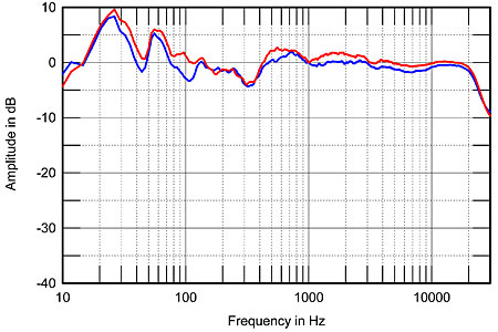
Fig.8 Aerial Acoustics 20T V2, spatially averaged, 1/6-octave response in JA's listening room, as initially (blue) and as finally (red) set up.

I don't normally measure loudspeaker distortion, but a potential problem with area-driven diaphragms such as ribbons, magnetic planars, and electrostatics is that they can generate subharmonics. Even at high levels, however, the Aerial ribbon tweeter's output was free from lower-frequency spuriae. It was also very low in conventional harmonic distortion. A 5kHz tone at a level of 80dB had the second harmonic at just –63dB (0.07%), and the third at –76dB (0.015%). This is better linearity than some power amplifiers!

The 20T V2's step response on the tweeter axis (fig.9) reveals that all the drive-units are connected with positive acoustic polarity. Although the tweeter's step leads that of the midrange unit, which in turn leads that of the woofers, the decay of each drive-unit's step smoothly blends into the step of the next lower in frequency, suggesting optimal crossover design. The Aerial's cumulative spectral-decay plot on the tweeter axis (fig.10) is superbly clean in the region covered by the ribbon tweeter—this is, indeed, an exceptional drive-unit. The decay of the sound is not quite as clean in the region handled by the midrange unit, but is still good in absolute terms. There is a slight ridge of delayed energy associated with the response step at the top of the midrange unit's passband, which, all things being equal, might be the cause of the slight nasal coloration I noticed in my auditioning.

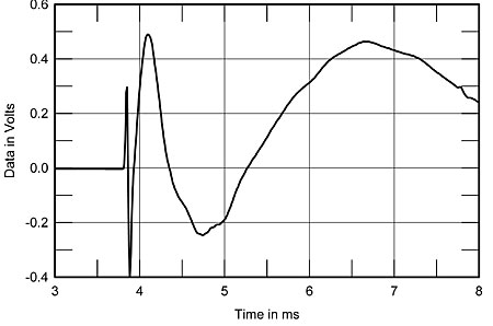
Fig.9 Aerial Acoustics 20T V2, step response on tweeter axis at 50" (5ms time window, 30kHz bandwidth).

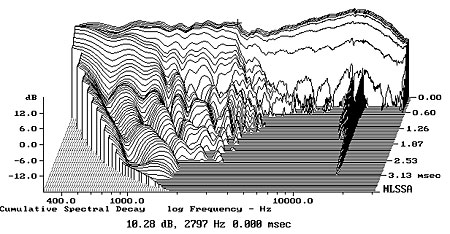
Fig.10 Aerial Acoustics 20T V2, cumulative spectral-decay plot on tweeter axis at 50" (0.15ms risetime).

That the Aerial 20T V2's measured performance is almost beyond reproach indicates some serious speaker engineering.—John Atkinson