Stand Loudspeaker Reviews

I use a mixture of nearfield, in-room, and quasi-anechoic FFT measurement techniques (using primarily DRA Labs' MLSSA system with a B&K 4006 microphone calibrated to be flat when used on-axis up to 30kHz—see "Follow-Up," October 1991, Vol.14 No.10—plus an Audio Control Industrial SA-3050A 1/3-octave spectrum analyzer with its own microphone) to investigate factors that might explain the sound heard. The impedance phase and amplitude of the speakers were measured using the magazine's Audio Precision System One.

Looking first at the manner in which the AE3's impedance magnitude and phase change with frequency (fig.1), the double hump in the bass is typical of a reflex design, with the 6.6 ohm minimum at 33Hz revealing the tuning of the four ports. With an impedance dropping to 3.1 ohms at 110Hz and 3750Hz, coupled with a relatively low sensitivity (I measured approximately 86dB/2.83V/m at 1kHz), the AE3 needs to be driven with an amplifier capable of swinging both volts and amps. Note the slight wrinkle in both amplitude and phase traces at 180Hz. Such behavior always indicates some kind of resonant problem. (The similar wrinkle just below 27kHz is due to the tweeter's "oil-can" diaphragm resonance, for example.) I thought at first that this corresponded with a cabinet resonance, but this turned out not to be the case. With the exception of sidewall vibrational modes at 230Hz and 410Hz and a rear-wall mode at 260Hz, the cabinet was well-damped. Sweeping a sinewave rapidly from 100Hz to 1kHz and listening to the cabinet output with a stethoscope, however, did reveal an internal metallic-sounding "honk," which might well correlate with the thickened upper-bass sound.

Fig.1 Acoustic Energy AE3, electrical impedance (solid) and phase (dashed). (2 ohms/vertical div.)

While doing these investigations, I was surprised to find the stand's bottom plate to vibrate strongly at 125, 230, and 260Hz. Sitting on the upward-pointing spikes, the speaker couples energy very efficiently to the stand and floor. It might be worth AE3 owners experimenting with different methods of coupling the speaker to the stand, therefore, to get the maximum lower-midrange transparency.

To look at a speaker's frequency response, I take five impulse responses with the MLSSA system across a 30° horizontal arc in front of the speaker on the tweeter axis. The impulse response actually on the AE3's HF axis with the grille removed is shown in fig.2: underneath the high-frequency ringing of the tweeter can be seen a fairly lazy decay pattern, due to the high-order crossover filters used. The step response is shown in fig.3. This indicates that all three drive-units are connected with positive polarity, but that the speaker is not time-coincident.

Fig.2 Acoustic Energy AE3, impulse response on tweeter axis at 45" (5ms time window, 30kHz bandwidth).

Fig.3 Acoustic Energy AE3, step response on tweeter axis at 45" (5ms time window, 30kHz bandwidth).

To calculate a loudspeaker's anechoic frequency response, the portion of each impulse response that is free from room reflections is transformed to the frequency domain with the mathematical aid of the Discrete Fourier Transform algorithm. The five amplitude responses are averaged, which minimizes the effect of microphone-position–dependent interference effects. The result is shown to the right of fig.4. While the overall trend is pretty flat but slightly down-tilted, from the lower midrange to 10kHz or so, a number of peaks and dips can be seen. What the audible effect of this behavior will be is hard to say (which is why we listen, of course). Note, however, the dip at the upper crossover frequency and the shelving-down of the top audio octave, from 10kHz to 20kHz, just below the very high tweeter resonance peak at 26.8kHz. The latter undoubtedly contributes to the AE3's somewhat "mellow" tonal balance.

Fig.4 Acoustic Energy AE3, anechoic response on tweeter axis at 45", averaged across 30° horizontal window and corrected for microphone response, with the nearfield responses of the woofer and port, plotted in the ratios of the square roots of their radiating areas below 300Hz and 1kHz, respectively.

To the left of fig.4 are shown the individual responses of the woofer and ports, measured in the nearfield (with the microphone capsule almost touching the diaphragm for the woofer and centered in one of the port openings). The matching in level between these traces and the quasi-anechoic trace to their right is my best guesstimate. As expected from fig.1, the maximum output from the port is centered on 33Hz, which corresponds to the minimum woofer output, revealed by the notch in its trace. (Remember that below this frequency, the output of the woofer is out of phase with that from the ports, doubling the rate of rollout.) Although not shown here, the woofer trace features a notch at 180Hz, as does that of the ports (which is shown). Again, this behavior may very well correlate both with the wrinkle at the same frequency seen in fig.1 and the speaker's lack of clarity in the upper bass, the feeling of detachment noted between the bass and lower midrange.

The way in which a speaker's sound changes as the listener moves off-axis is important in that it affects both the reverberant soundfield in the room and the sound of the first reflections of the speaker's direct sound from the sidewalls. This is shown in fig.5, which shows the differences between the on-axis sound and that measured to the side of that axis. As well as the extreme high frequencies rolling off the more off-axis the listener gets, a peak develops between 1 and 2kHz, which would make the in-room sound in all but very dead rooms a little bright.

Fig.5 Acoustic Energy AE3, lateral response family at 45", normalized to response on tweeter axis, from back to front: differences in response 30–7.5° off axis, reference response, differences in response 7.5–90° off axis.

Carrying out the same exercise for vertical listening height gives the family of curves shown in fig.6, which again shows the differences between the various responses and that on the tweeter axis. By comparing fig.6 with fig.4, it can be seen that listening too low—the front two traces—gives an even deeper crossover suckout. In fact, the optimum balance seems to be with the listener's ears level with the top of the cabinet, when the various holes and peaks in fig.4 will flatten out. This axis, however, is 44" from the ground, which represents a very high listening chair. Remember that with my listening chair placing my ears 36" from the ground, I found it beneficial to tilt the speaker stands forward a little.

Fig.6 Acoustic Energy AE3, vertical response family at 45", normalized to response on tweeter axis, from back to front: differences in response 15–7.5° above axis, reference response, differences in response 7.5° below axis.

To see how these quasi-anechoic measurements translate to the in-room balance, I perform 10 1/3-octave spectrum analyses of pink noises for left and right speakers individually in a 72" by 20" "window" around the listening position. Averaging these spectra minimizes the effects of room standing waves and gives a curve reflecting the mix of the speakers' direct sound and the reverberant soundfield in the listening room. That for the AE3 is shown in fig.7. The useful bass extends to below 35Hz while the generally smooth response trend is broken only by residual steady-state room effects (the peak at 63Hz and dip between 200Hz and 400Hz) and a slight excess of energy centered on 2kHz. The gentle slope from 500Hz to 10kHz should give the speaker a musically natural tonal balance, broken only by some brightness due to the 2kHz prominence, while the drop in energy above 10kHz again will render the AE3's sound rather too mellow for some tastes.

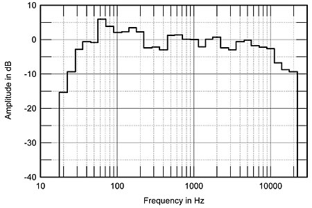
Fig.7 Acoustic Energy AE3, spatially averaged, 1/3-octave response in JA's Santa Fe listening room.

Finally, taking the impulse response of fig.2 and performing a series of Fourier Transforms beginning at successively delayed starting points shows how the speaker's frequency response changes as the sound decays. Any resonances present will manifest themselves as ridges parallel to the graph's time axis, as the sound will take longer to decay at these frequencies. This cumulative spectral-decay or "waterfall" plot for the AE3 is shown in fig.8. Apart from the high-level tweeter resonance at 27kHz obvious at the right-hand side of the graph, a second resonance can be seen at 4.6kHz (the cursor position), most probably the first breakup mode of the midrange unit's metal diaphragm, and a third an octave higher but much lower in level. The main mode is 1kHz lower in frequency than the similar metal-cone resonance featured by the midrange/woofer in Monitor Audio's Studio 20 loudspeaker reviewed by RH in the December 1991 issue, which might explain why it was more audible. There is nothing visible around 1kHz which would correspond with the off-axis peak noted in fig.6, but the obvious discontinuity in the sound at 2kHz suggests that something peculiar is going on in this region, which might again add a feeling of brightness to the speaker's balance.—John Atkinson

Fig.8 Acoustic Energy AE3, cumulative spectral-decay plot on tweeter axis at 45" (0.15ms risetime).